9. Examples of Relativity in Action

In this chapter we will explore how to use the energy-momentum four vector to understand three example situations. First, in the collision of two particles, how much energy is available to potentially create more particles? Second, how to apply the Lorentz transformation to the momentum four vector when the particle in the system is a photon? And finally, what happens to the energy of a photon when it collides with (also called “scatters off of”) a free electron?

9.1. The Center of Momentum Frame

The traditional scattering experiment that physicists use to probe the nature of the interaction between pieces of a system is typically done in a laboratory where one particle is accelerated and smashed into a stationary target particle. The energy, momentum, etc. of the debris from the interaction are then measured. Other scattering experiments use colliding beams, where two beams of particles traveling in opposite directions are allowed to interact. While this gives more energy to do interesting things, the probability of interactions occuring are smaller.

In the simplest case, there is one incident particle (with a rest energy of \(E_{0i}\), but moving with a momentum \(p_i\) and a kinetic energy of \(KE_i\)) and one target particle (at rest, with a rest energy of \(E_{0t}\)) that interact in a particular place at a particular time. Take the \(x\) axis to be parallel to the momentum vector of the incident particle. Then we can write the four-momentum of the incident particle as

(9.1)\[\begin{split}[p_4]_i = \begin{bmatrix} i(E_{0i} + KE_i)/c\\ p_i\\ 0\\ 0 \end{bmatrix}\end{split}\]

and the four-momentum of the target particle is

(9.2)\[\begin{split}[p_4]_t = \begin{bmatrix} iE_{0t}/c\\ 0\\ 0\\ 0 \end{bmatrix}\end{split}\]

The total 4-momentum for the scattering as determined by an observer in the laboratory reference frame is (writing the incident momentum in terms of the KE using Equation (8.20)):

(9.3)\[\begin{split}[p_4]_{\rm lab} = \begin{bmatrix} i\frac{1}{c}(E_{0i} + KE_i + E_{0t})\\ \frac{1}{c}\sqrt{KE_i^2 + 2 E_{0i}KE_i}\\ 0\\ 0 \end{bmatrix}\end{split}\]

When the scattering interaction happens, new particles can be formed, but the momentum 4-vector describing the system remains constant (is conserved) as long as you stay in the same inertial reference frame. All of the appropriate quantum numbers must also be conserved, e.g. charge, baryon number, etc.

Suppose that there is a second observer, watching this same scattering process take place. This observer is moving in the same direction as the incident particle, but at a slower speed. This observer sees the incident particle moving slower, but now the target particle has some physical momentum that is pointing in the opposite direction that the observer is traveling.

At some relative speed \(\beta_{\rm com}\) the second observer will measure the incident particle and the ‘target’ particle to have the same size physical momentum, but pointing in opposite directions. The total physical momentum in this case is 0. This reference frame is known as the zero-momentum or center-of-momentum (com) reference frame. The 4-momentum for this frame is:

(9.4)\[\begin{split}[p_4]_{\rm com} = \begin{bmatrix} iE_{\rm com}/c\\ 0\\ 0\\ 0 \end{bmatrix}\end{split}\]

The center-of-momentum frame is a very special case. After the interaction takes place, the physical momentum of all of the particles still must equal 0. If this scattering process were to make different particles than the two incident particles, the threshold (the lowest energy at which it could occur) would have the new particle produced each with 0 momentum (and KE). This means that \(E_{\rm com}\) is the maximum energy available to make new particles in the interaction. We say maximum because the KE of the daughter particles won’t actually be zero in a real situation. If the two parent particles survive the interaction, their rest mass must be accounted for out of the total energy, too. The value \(E_{\rm com}\) is a budget of energy that must be allocated to the rest energies and kinetic energies of everything that comes out of the interaction.

The time component of the 4-momentum in the com reference frame (the total energy in the center-of-momentum) tells which new particles can be produced in a scattering reaction. If there is any energy left over after creating the rest energies of the new particles, it goes into the kinetic energy of the new particles. The kinetic energy is distributed in such a way that the total physical momentum of the particles is 0.

If the 4-momentum in the lab is known, then the 4-momentum in the com frame can be found using the Lorentz transformation:

(9.5)\[[p_4]_{\rm com} = {\cal L}_x (\beta_{\rm com})[p_4]_{\rm lab}\]

Plugging in Equation (9.3) (and ignoring \(y\) and \(z\)) we get

(9.6)\[\begin{split}[p_4]_{\rm com} = \begin{bmatrix} \gamma_{\rm com} & -i\beta_{\rm com}\gamma_{\rm com} \\ i\beta_{\rm com}\gamma_{\rm com} & \gamma_{\rm com} \\ \end{bmatrix} \begin{bmatrix} i\frac{E_{\rm lab}}{c}\\ p_i\\ \end{bmatrix}\end{split}\]

Matrix multiplication yields:

(9.7)\[\begin{split}\begin{bmatrix} iE_{\rm com}/c\\ 0 \end{bmatrix} = \gamma_{\rm com} \begin{bmatrix} i(E_{\rm lab}/c-\beta_{\rm com}p_i)\\ p_i-\beta_{\rm com}E_{\rm lab}/c\\ \end{bmatrix}\end{split}\]

The second row of Equation (9.7) tells how to find the relative speed of the com reference frame if you know the total energy and momentum in the lab reference frame. The two terms must cancel, if the total momentum is to be zero, and that can only happen if

(9.8)\[\boxed{ \beta_{\rm com} = \frac{cp_i}{E_{\rm lab}} = \frac{\sqrt{KE_i^2 + 2 E_{0i}KE_i}}{E_{0i} + KE_i + E_{0t}}}\]

There really isn’t any further simplification one can do to Equation (9.8). Every quantity on the right would be known as inputs for a given experiment, so you could calculate the necessary speed of the com for any target particle being hit by any incident particle with any kinetic energy you choose.

We can, however, apply a limit check and consider what happens as the KE of the incident particle gets very, very large. In such a limit, the rest energies become negligible and \(\beta_{\rm com} \rightarrow 1\). This makes sense because the faster the incident particle is going, the closer its speed gets to one, the more it dominates the sum that makes up the total momentum, so effectively the target plays no role, and the com is going right along with the incident particle.

If the target and the incident particle are the same kind of particle, such that \(E_{0i}=E_{0t}\equiv E_0\), then we can do one further simplification – pull out a \(\sqrt{KE_i}\) in the numerator:

(9.9)\[\beta_{\rm com} = \sqrt{KE_i} \frac{\sqrt{KE_i + 2 E_0}}{KE_i + 2E_0} = \sqrt{\frac{KE_i}{KE_i + 2E_0}} = \left(1+\frac{2E_0}{KE_i}\right)^{-1/2}\]

In this case you can see, again, that as \(KE_i\) gets large, \(\beta_{\rm com}\rightarrow 1\), but it’s easier to see.

The first row of Equation (9.7), on the other hand, tells us the total energy available in the com frame:

(9.10)\[E_{\rm com} = \gamma_{\rm com}(E_{\rm lab} - \beta_{\rm com} c p_i)\]

The fact that we are subtracting something from \(E_{\rm lab}\) on the right side of Equation (9.10) makes it look like the amount of energy in the com frame is less than the amount of energy in the lab frame, but you have to be cautious with such generalizations, because \(\gamma_{\rm com}\) is also getting larger as \(p_i\) increases, so it’s not so trivial to see which effect will dominate.

However, Fig. 9.1 shows how much energy is available in the COM frame, according to Equation (9.10) (after subtracting off the rest energies of the original two particles) as a function of how much kinetic energy the incident particle has. You can see that the amount of available energy is significantly less than the amount of KE put in (the black dotted line represent equality). It appears that some of the energy in the lab frame goes into moving the center of momentum of the system.

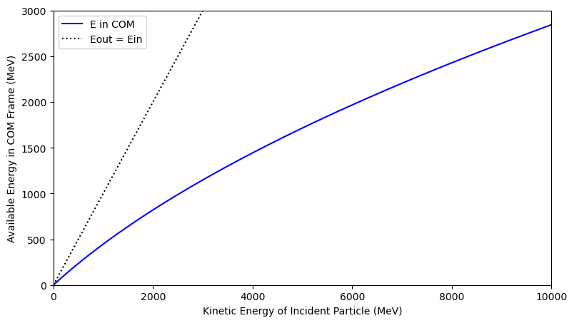
Fig. 9.1 Graph of energy available in the COM frame (after subtracting the rest energy of the two particles involved) as a function of the KE of the incident particle in the lab frame. There is significantly less energy available in the COM frame to make particles than in the lab frame, if you put all the KE into accelerating one particle at the stationary target.

9.1.1. Example 9.1

A proton with kinetic energy 300.00 MeV strikes a stationary proton. Find the speed of the center-of-momentum frame and the total energy in the center-of-momentum frame. Is it possible for this scattering process to produce two pions?

Tofind the speed of the center-of-momentum, we use Equation (9.8). The total energy in the laboratory frame is

\[E_{\rm labtot} = 938.26~{\rm MeV}+ 300.00~{\rm MeV}+ 938.26~{\rm MeV} = 2176.52~{\rm MeV}\]

The incident proton has all of the momentum in the lab reference frame, so

\[cp_i =\sqrt{2(938.26~{\rm MeV})(300~{\rm MeV}) + (300~{\rm MeV})^2} \rightarrow p_i = 808.06~{\rm MeV}/c\]

The momentum 4-vector for the system in the laboratory frame is:

\[\begin{split}[p_4]_{\rm lab} = \begin{bmatrix} i 2176.52~{\rm MeV}/c\\ 808.06~{\rm MeV}/c\\ 0.0\\ 0.0 \end{bmatrix}\end{split}\]

The speed of the com frame is found using Equation (9.8):

\[\beta_{\rm com} = \frac{808.26}{2176.52} = 0.37135\]

To find the energy available to make new particles, we use Equation (9.10). First, find \(\gamma_{\rm com}\) from \(\beta_{\rm com}\):

\[\gamma_{\rm com} = \frac{1}{\sqrt{1-\beta_{\rm com}^2}} = 1.0770\]

Then plug into Equation (9.10):

\[E_{\rm com} = 1.0770\left((2176.52~{\rm MeV}) - 0.37135(808.26~{\rm MeV})\right) = 2020.85~{\rm MeV}\]

The rest energy of the charged pions is 139.6 MeV and the neutral pion has restenergy 135.0 MeV. It would seem that you could make a lot of pions. However, charge and baryon number must also be conserved. In the lab, we started with two baryons, so some of this energy must go into making two more baryons. The baryon with the lowest rest energy is the proton, so if we make two protons, there is 2020.85 MeV- 1876.52 MeV = 144.33 MeV left over. This energy could go into the kinetic energy of the two protons (the collision would then just be called elastic scattering), or it could be used to make 1 neutral pion. The two protons and the neutral pion would share the leftover 9.3 MeV of energy as kinetic energy. This energy would be distributed in such a way that the total physical momentuin of the three particles would be zero (in the COM frame, of course. In the lab, the total momentum of the three particles would be the same as the original momentum of the incident proton).

9.1.2. Example 9.2

The first strange particles to be produced were the \(\Lambda^0\) and the \(K^0\) They were produced by colliding a high energy (large kinetic energy) negative pion with a stationary proton in a bubble chamber. What is the minimum kinetic energy that the pion must have if the interaction is to produce these two strange particles?

In this case, we work backwards from knowing what the the minimum energy in the center-of-momentum frame would be. It must be at least the sum of the rest energies of the two particles to be produced.

\[E_{\rm commin} = E_{0\Lambda} + E_{0K} = 1115.7~{\rm MeV} + 497.7~{\rm MeV} = 1613.4~{\rm MeV}\]

Transforming the momentum 4-vector in the com frame back into the lab frame gives

(9.11)\[\begin{split}\begin{bmatrix} i\frac{E_{\rm tot}}{c}\\ p_x\\ \end{bmatrix} = \begin{bmatrix} \gamma_{\rm com} & i\beta_{\rm com}\gamma_{\rm com} \\ -i\beta_{\rm com}\gamma_{\rm com} & \gamma_{\rm com} \end{bmatrix} \begin{bmatrix} i\frac{E_{\rm commin}}{c}\\ 0.0 \end{bmatrix}\end{split}\]

We can use Equation (8.20) to write \(p_x\) as \(\sqrt{E_{0\pi}KE_\pi + KE_\pi^2}\) and the total energy is \(E_{0\pi} + E_{0p} + KE_\pi\). That covers the left side of Equation (9.11) and the only unknown there is the KE of the pion. On the right side, we multiply out the matrix to get

(9.12)\[\begin{split}\begin{bmatrix} i\frac{E_{0p}+E_{0\pi}+KE_\pi}{c}\\ \frac{1}{c}\sqrt{E_{0\pi}KE_\pi + KE_\pi^2}\\ \end{bmatrix} = \begin{bmatrix} \gamma_{\rm com} i\frac{E_{\rm commin}}{c}\\ \beta_{\rm com}\gamma_{\rm com}\frac{E_{\rm commin}}{c} \end{bmatrix}\end{split}\]

If you include the definition of \(\gamma_{\rm com}\), that’s three equations and three unknowns (\(KE_\pi\), \(\beta_{\rm com}\), and \(\gamma_{\rm com}\)), so we can solve for an answer!

(9.13)\[E_{0p} + E_{0\pi} + KE_\pi = \gamma_{\rm com}E_{\rm commin}\]

(9.14)\[E_{0\pi}KE_\pi + KE_\pi^2 = \beta_{\rm com}^2\gamma_{\rm com}^2E_{\rm commin}^2\]

and of course

(9.15)\[\gamma_{\rm com} = \frac{1}{\sqrt{1-\beta_{\rm com}^2}}\rightarrow \beta_{\rm com}^2 = 1-\frac{1}{\gamma_{\rm com}^2}\]

Remember what we are looking for is \(KE_\pi\), and we know \(E_{commin}\) and the rest energies. From here on, it’s basically algebra. Put Equation (9.15) into Equation (9.14) to get

(9.16)\[E_{0\pi}KE_\pi + KE_\pi^2 =(\gamma_{\rm com}^2-1)E_{\rm commin}^2\]

solve for \(\gamma_{\rm com}^2E_{\rm commin}^2\) to get

(9.17)\[\gamma_{\rm com}^2E_{\rm commin}^2 = E_{0\pi}KE_\pi + KE_\pi^2 +E_{\rm commin}^2\]

Square Equation (9.13) and plug in Equation (9.17) to get

(9.18)\[(E_{0p} + E_{0\pi} + KE_\pi)^2 = \gamma_{\rm com}^2E_{\rm commin}^2 = E_{0\pi}KE_\pi + KE_\pi^2 +E_{\rm commin}^2\]

Looks like a mess, but terms are going to cancel. Expand the square on the left side:

(9.19)\[(E_{0p} + E_{0\pi})^2 + 2(E_{0p} + E_{0\pi})KE_\pi + KE_\pi^2 = E_{0\pi}KE_\pi + KE_\pi^2 +E_{\rm commin}^2\]

The \(KE_\pi\) square term cancels! Then it’s simple to solve for \(KE_\pi\):

(9.20)\[KE_\pi(2(E_{0p} + E_{0\pi})- E_{0\pi}) = -(E_{0p} + E_{0\pi})^2 +E_{\rm commin}^2\]

Divide through to get

(9.21)\[KE_\pi = \frac{E_{\rm commin}^2 - (E_{0p} + E_{0\pi})^2}{2E_{0p} + E_{0\pi}}\]

We can plug in numbers to this equation and get

E0p = 938.28
E0pi = 139.570 
Ecommin = 1613.4
KEpi = (Ecommin**2-(E0p+E0pi)**2)/(2*E0p+E0pi)
print("Minimum KE of pion: {:5.2f} MeV".format(KEpi))

Minimum KE of pion: 714.88 MeV

So in the lab, we have 715 MeV of kinetic energy with the pion, plus the rest energy of the pion (140 MeV) and the rest energy of the proton (938 MeV), for a total of 1793 MeV of energy. Assuming we did the math correctly, that must correspond to 1613 MeV of energy in the center of momentum frame, which would be enough to make the two particles. So we would need more energy in the lab than you might think, to ensure we had enough energy in the center of momentum frame. If an event (like the creation of two new particles) is to happen in one frame, then it must happen in all frames. Specifically, if there is not enough energy in the CoM frame for the particles to be created, then they cannot be created in ANY frame. So in the lab, the pion must have 715 MeV of kinetic energy to ensure there is enough energy in the CoM frame, even though it is more than enough energy in the lab frame.

9.2. Photons and the Doppler Shift

The Doppler shift tells what happens to the measured energy of a photon when it is viewed by different inertial observers. The velocity of the photon is the same for both inertial observers, but the energy changes. The momentum 4-vector for a photon as seen by the first observer is

(9.22)\[\begin{split}[p_4]_1 = \begin{bmatrix} iE_1/c\\ E_1/c\\ 0\\ 0 \end{bmatrix} = \begin{bmatrix} ih/\lambda_1\\ h/\lambda_1\\ 0\\ 0 \end{bmatrix}\end{split}\]

where we use \(E=hf\) and \(c=\lambda f\) to get the latter form.

Notice that the size of the momentum 4-vector for a photon (or any zero rest energy particle) is 0. That is because the size of the momentum 4-vector = \(-m_0c^2\), and the particle does not have any rest energy.

A second inertial observer moving with \(\beta_R\) in the \(+x\) direction with respect to the first inertial observer, watching this same photon, would measure a momentum 4-vector given by (again ignoring \(y\) and \(z\)):

(9.23)\[\begin{split}[p_4]_2 = \begin{bmatrix} iE_2/c\\ E_2/c \end{bmatrix} = \begin{bmatrix} \gamma_R & -i\beta_R\gamma_R \\ i\beta_R\gamma_R & \gamma_R \\ \end{bmatrix} \begin{bmatrix} iE_1/c\\ E_1/c \end{bmatrix} = \gamma_R \begin{bmatrix} i(E_1/c-\beta_RE_1/c)\\ E_1/c-\beta_RE_1/c \end{bmatrix}\end{split}\]

So

(9.24)\[\begin{split}[p_4]_2 = \begin{bmatrix} iE_2/c\\ E_2/c \end{bmatrix} = E_2/c \begin{bmatrix} i\\ 1 \end{bmatrix} = \gamma_RE_1(1-\beta_R)/c \begin{bmatrix} i\\ 1 \end{bmatrix}\end{split}\]

The part in brackets is clearly the same, so \(E_2=\gamma_R(1-\beta_R)E_1\). Plug in the definition of \(\gamma_R\) to get

(9.25)\[E_2 = E_1 \frac{1-\beta_R}{\sqrt{1-\beta_R^2}} = E_1 \frac{1-\beta_R}{\sqrt{(1-\beta_R)(1+\beta_R)}} = E_1\sqrt{\frac{1-\beta_R}{1+\beta_R}}\]

\[\boxed{ E_2 = E_1\sqrt{\frac{1-\beta_R}{1+\beta_R}} }\]

Since \(\beta_R\leq 1\), the numerator in Equation (9.25) will always be less than the denominator, so as long as the second observer is moving to the right (receding from the source of the light), she will measure a smaller energy than the first observer would. If the second observer switches direction and heads toward the source of light, the \(\beta\) will change sign, which effectively flips the ratio under the square root. In that case, \(E_2\geq E_1\) – the energy goes up.

This is qualitatively not different from the case of a massive particle: if you throw a ball at me, and I run toward you, the ball will have more energy in my reference frame. If I run away, the ball will have less energy. However, for a massive object like a ball or a proton, that energy is associated with speed. For a massless particle like a photon, the speed does not change – it always moves at \(c\). The energy in that case is associated with the frequency (or equivalently, the wavelenth) of the light. So, for light, we often write Equation (9.25) in terms of frequency (\(f\)) or wavelength (\(\lambda\)):

(9.26)\[\boxed{ f_2 = f_1\sqrt{\frac{1-\beta_R}{1+\beta_R}}}\]

and

(9.27)\[\boxed{ \lambda_2 = \lambda_1\sqrt{\frac{1+\beta_R}{1-\beta_R}}}\]

Since \(\lambda = c/f\), these two equations are reciprocals.

Since Equation (9.26) says the photons will be shifted toward smaller frequencies if the relative velocity of the source and observer is positive (receding), and the smallest frequencies of visible light are red, we refer to this kind of change as a “redshift”, and if the source and receiver are approaching (negative relative velocity), we call this change a “blueshift”. This can be confusing if you are considering photons outside the visible range of light. An x-ray, for example, subject to a blueshift, changes to an even higher frequency, away from blue light on the electromagnetic spectrum. So if the “blue” and “red” confuse you, just think of going to higher or lower frequency (which means going the opposite direction in wavelength).

Warning

It doesn’t make sense to ask whether the source or the receiver is “really” moving, because all motion is relative. For a sound wave, the medium it moves through provides a context in which it might make sense to say one or the other is “really” moving (relative to the medium), but in Chapter 1 we showed that the Michelson Morely experiment disproves the hypothesis that light has a medium. So any motion of source or receiver is equivalent and indistinguishable.

9.3. Compton Scattering

9.3.1. Experimental Background

Photon-electron scattering, called Compton scattering [Compton, 1923], was proposed by Arthur Compton as a way of finding out if the relativistic model of a photon having a momentum \(p=E/c\) was valid. It seemed impossible that a particle with no mass (zero rest energy) could have momentum.

Compton shot 17.5 keV X-ray photons at a carbon target as schematically shown on the left side of Fig. 9.2. If the relativistic model were not wrong, the photons would interact with the valence electrons (those that are not tightly bound to the nucleus, typically 11 eV binding energy) in the atom. According to relativity, the interaction should be similar to that of billiard balls colliding. The valence electron would get scattered at some angle \(\phi\) and the scattered photon would be emitted at some other angle \(\theta\) as schematically shown on the right side of Fig. 9.2.

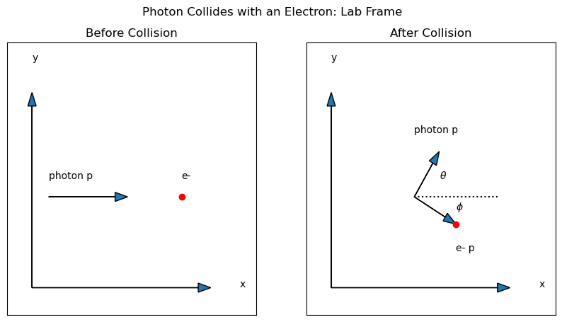
Fig. 9.2 Schematic diagram of a photon scattering off of an electron within the frame of reference of the laboratory. The left side shows the situation before the collision, while the right side shows the scattering after the collision. Note that these are NOT spacetime diagrams. Both axes are spatial dimensions. The arrows represent momentum. Before the collision, the electron (red dot) is at rest and the \(x\) axis is chosen to align with the incoming photon momentum. After the collision, the photon is traveling with an angle \(\theta\) with regards to the horizontal, while the electon now has a momentum, and is moving with an angle \(\phi\) below the horizontal. The sum of the momenta of the photon and the electron after the collision is equal to the momentum of the photon before the collision.

The energy and momenta of the scattered particles would be determined by momentum and energy conservation. Compton worked out the theory for the scattering and did the experiment. He measured the energy of the scattered photons as a function of angle \(\theta\). The theory and experiment were in beautiful agreement, giving a clear confirmation of the relativistic theory. For this work, Arthur Compton was awarded the 1927 Nobel Prize in physics.

9.3.2. Special Relativistic Model

In the laboratory frame (Fig. 9.2), the momentum 4-vector for the system is

(9.28)\[\begin{split}[p_4]_{\rm lab} = \begin{bmatrix} i\frac{1}{c}(E_{\rm phot} + E_{0})\\ \frac{E_{\rm phot}}{c}\\ 0\\ 0 \end{bmatrix}\end{split}\]

where \(E_0\) is the rest energy of the electron and \(E_{\rm phot}/c\) is the momentum of the photon.

I am not going to ignore \(y\) and \(z\) for this problem, because we will need to consider the motion of the particles in the \(y\) direction.

We then use Equation (9.8) to find the speed of the center of momentum frame \(\beta_{\rm com}\):

(9.29)\[\boxed{ \beta_{\rm com} = \frac{E_{\rm phot}}{E_{\rm phot} + E_0}}\]

If we switch into this frame (left side of Fig. 9.3), the two particles will both be heading toward each other. Not at the same speed, of course (the photon is still moving at the speed of light), but with the same momentum.

Now, we can use the results from the Doppler shift (Equation (9.25)) to find the energy of the photon before the collision in the com reference frame.

(9.30)\[E_{\rm photcom} = \gamma_{\rm com}(1-\beta_{\rm com})E_{\rm phot}\]

After the collision in the COM frame (see the right side of Fig. 9.3), the scattered photon and the recoiling electron still must have a total momentum of 0 and the same total energy as before the collision. The only way for this to happen at any angle \(\xi\) for the two scattered particles to have the same size momentum as they did before the collision.

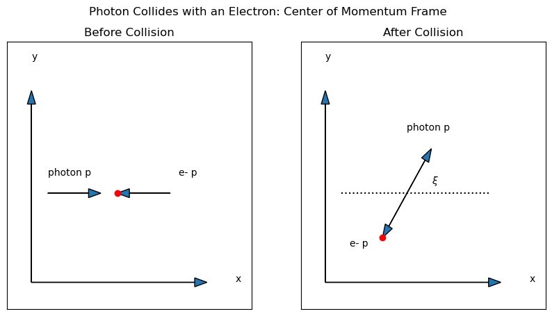
Fig. 9.3 Schematic diagram of a photon scattering off of an electron within the center of momentum frame of reference. The left side shows the situation before the collision, while the right side shows the scattering after the collision. Note that these are NOT spacetime diagrams. Both axes are spatial dimensions. The arrows represent momentum. Before the collision, the electron (red dot) has a momentum equal and opposite to the photon momentum. After the collision, the photon and the electron both still have equal and opposite momentum, but the angle of their motion has changed completely. The photon now makes an angle of \(\xi\) with the horizontal axis.

So after the collision, the energy of the scattered photon is still the same as in Equation (9.30). It is just going out at an angle \(\xi\) with respect to the x axis. The 4-momentum of this scattered photon is

(9.31)\[\begin{split}[p_4]_{\rm photcom~AFTER} = \begin{bmatrix} i\frac{E_{\rm photcom}}{c}\\ \frac{E_{\rm photcom}}{c}\cos{\xi}\\ \frac{E_{\rm photcom}}{c}\sin{\xi}\\ 0 \end{bmatrix}\end{split}\]

I am using \(E_{\rm phot}\) for the original energy of the incoming photon in the lab reference frame before the collision. \(E_{\rm photlab}\) is the energy of the outgoing photon after the collision in the lab reference frame. \(E_{\rm photcom}\) is the energy of the photon after the collision in the COM reference frame.

This is the same photon that is scattered at an angle \(\theta\) and has energy \(E_{\rm photlab}\) in the laboratory reference frame (after the collision). The 4-momentum for this same photon in the laboratory frame after the scattering is

(9.32)\[\begin{split}[p_4]_{\rm phot~AFTER} = \begin{bmatrix} i\frac{E_{\rm photlab}}{c}\\ \frac{E_{\rm photlab}}{c}\cos{\theta}\\ \frac{E_{\rm photlab}}{c}\sin{\theta}\\ 0 \end{bmatrix}\end{split}\]

As you might suspect, the way to connect these two four vectors is through a Lorentz transformation!

(9.33)\[\begin{split}\begin{bmatrix} i\frac{E_{\rm photcom}}{c}\\ \frac{E_{\rm photcom}}{c}\cos{\xi}\\ \frac{E_{\rm photcom}}{c}\sin{\xi}\\ 0 \end{bmatrix} = \begin{bmatrix} \gamma_{\rm com} & -i\beta_{\rm com}\gamma_{\rm com} & 0 & 0\\ i\beta_{\rm com}\gamma_{\rm com} & \gamma_{\rm com} & 0 & 0\\ 0 & 0 & 1 & 0\\ 0 & 0 & 0 & 1 \end{bmatrix} \begin{bmatrix} i\frac{E_{\rm photlab}}{c}\\ \frac{E_{\rm photlab}}{c}\cos{\theta}\\ \frac{E_{\rm photlab}}{c}\sin{\theta}\\ 0 \end{bmatrix}\end{split}\]

Multiplyting out the time component yields

(9.34)\[E_{\rm photcom} = \gamma_{\rm com} E_{\rm photlab}(1-\beta_{\rm com}\cos{\theta}) = \gamma_{\rm com}(1-\beta_{\rm com})E_{\rm phot}\]

where the rightmost term is the energy of the photon before the collision, in the lab frame.

The factors of \(\gamma_{\rm com}\) cancel, and we can substitute in Equation (9.29) for \(\beta_{\rm com}\) to get

(9.35)\[E_{\rm photlab}\left(1- \frac{E_{\rm phot}}{E_{\rm phot} + E_0}\cos{\theta}\right) = \left(1- \frac{E_{\rm phot}}{E_{\rm phot} + E_0}\right)E_{\rm phot}\]

Find a common denominator to get rid of the ones:

(9.36)\[E_{\rm photlab}\left( \frac{E_0+E_{\rm phot}(1-\cos{\theta})}{E_{\rm phot} + E_0}\right) = \left(\frac{E_0}{E_{\rm phot} + E_0}\right)E_{\rm phot}\]

Cancel the denominator:

(9.37)\[E_{\rm photlab}\left( E_0+E_{\rm phot}(1-\cos{\theta})\right) = E_0E_{\rm phot}\]

This equation is usually written in a final form by dividing both sides by the triple product \(E_0E_{\rm phot}E_{\rm photlab}\) to get

(9.38)\[\boxed{ \frac{1}{E_{\rm photlab}} = \frac{1}{E_{\rm phot}} + \frac{1}{E_0} (1-\cos{\theta})}\]

Why would you want to write it like this? Well, first of all it gets each energy by itself instead of having three different products of two energies, so it’s simpler in that regard. More importantly, though, if you, like Compton, did an experiment where you varied \(\theta\) by placing your detector (which measures \(E_{\rm photlab}\)) at different angles, then you could make a plot where your horizontal axis is \((1-\cos{\theta})\) and your vertical axis is \(1/E_{\rm photlab}\), then you would expect to see a straight line relationship, where the y-intercept is not different from the known original value of \(1/E_{\rm phot}\). In which case you could interpret the slope of the line as giving you an estimate of \(1/E_0\), which would mean that the reciprocal of the slope would be an estimate of the rest energy of the electron!

Equation (9.38), which was derived assuming that the photon acts like a particle with momentum given by \(p=E/c\), demanding that physical momentum and total energy be conserved in any particular reference frame and using the Lorentz transformation to move between two different inertial reference frames, predicts this simple linear relationship between measured energy of the scattered photon (reciprocal) and the angle of the scattering (expressed as \(1-\cos{\theta}\)). We just need a linear plot to carry out the test!

Unfortunately, Arthur Compton’s Nobel Prize-winning 1923 paper does not actually include such a plot, but he does include the original spectra he recorded that show the energy shift for eight different values of \(\theta\). These graphs are copied here as Fig. 9.4. From these graphs, and the information given in the paper, it is possible to measure \(E_{\rm photlab}\) and construct the graph we need to test the hypothesis posed by Equation (9.38). Such a graph for four of the measurements reported in 1923 is shown in Fig. 9.5.

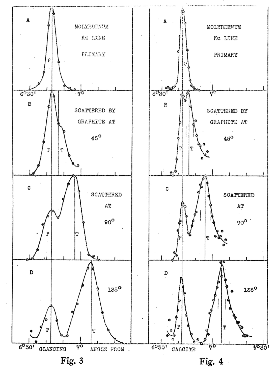
Fig. 9.4 Figures from Compton’s original 1923 paper. The intensity of X-rays is shown as a function of glancing scattering angle off a calcite crystal, which is proportional to energy. The graphs clearly show two peaks when the scattering angle is greater than zero, and the greater the angle of scattering, the more the second peak (T) shifts away from the first (P). The “P” peak is made of X-rays that scatter off the bound electrons in the crystal lattice, which therefore have much higher effective inertias, since they are attached to their nuclei. The free electrons can absorb the energy of the X-rays, and therefore these collisions result in the energy shift between T and P. Compton points out that the vertical lines are not averages, but the predictions of where the lines should be made by Equation (9.38).

The best linear fit parameters are calculated in the code that makes the graph, and displayed here:

# Linear fit results from Compton 1923
slp = b
icpt = a
E0=1/slp
Eg = 1/icpt
eslp = 3.51e-5
eicpt = 3.51e-5
eE0 = eslp*E0**2
eEg = eicpt*Eg**2
print("The best-fit slope is ({0:3.2f} +- {1:3.2f})x10^-3 1/keV".format(slp*1000,eslp*1000))
print("The best-fit y-intercept is ({0:4.3f} +- {1:4.3f})x10^-2 1/keV".format(icpt*100,eicpt*100))
print("The estimate of E0 is ({0:3.0f} +- {1:2.0f}) keV".format(E0,eE0))
print("The estimate of Egam is ({0:4.2f} +- {1:3.2f}) keV".format(Eg,eEg))

The best-fit slope is (1.90 +- 0.04)x10^-3 1/keV
The best-fit y-intercept is (5.712 +- 0.004)x10^-2 1/keV
The estimate of E0 is (526 +- 10) keV
The estimate of Egam is (17.51 +- 0.01) keV

Note the excellent agreement between experiment and the predictions of Equation (9.38)! One over the y-intercept is \(17.51\pm0.01\) keV, which is within one \(\sigma\) of the known 17.5 keV value for the incoming photons in the lab frame. Since the known value of the X-ray energy is critical in converting the angle in the figure to an energy, this is not surprising, but it is a nice self-consistency check. The best fit slope is the important result. The slope shown in Fig. 9.5 is \((1.90\pm0.04)\times10^{-3}\) 1/keV, which means the best estimate of the rest mass of the electron from this experiment is \(526\pm10\) keV. This is within 1.4 \(\sigma\) of the current accepted best value, 511 keV.

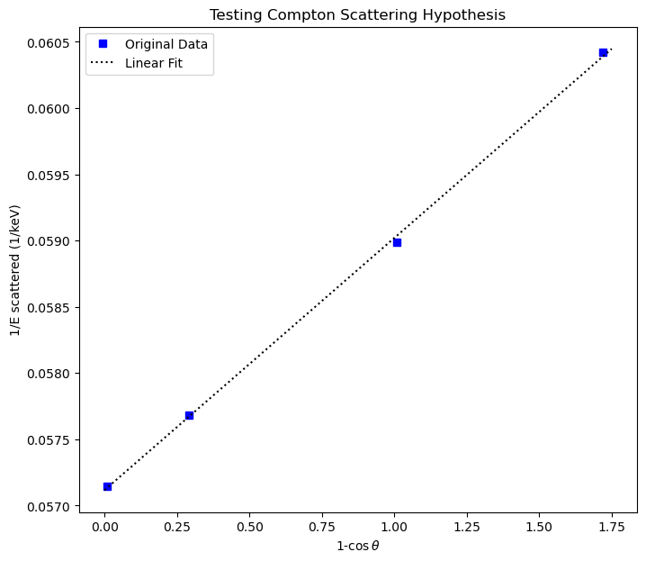
Fig. 9.5 Graph constructed from measurements reported in Compton’s 1923 paper. He measured the wavelength of 17.5 keV X-rays scattered from graphite. Notice the agreement with the predictions of Equation (9.38). The slope can be interpreted as 1/(rest energy of an electron).

9.4. Problems

1. A 500.0 MeV proton collides with a stationary neutron.

a) Determine the speed of the center-of-momentum frame for this system.

b) Determine the total energy in the center-of-momentum frame.

2. Find the laboratory threshold energy for this scattering reaction (when the proton is the incident particle hitting the stationary neutron):

\[p^+ + n^0 \rightarrow n^0 + n^0 + \pi^+\]

3. A 200 MeV anti-proton interacts with a stationary neutron in the lab and produces two pions

\[\bar{p}^- + n^0 \rightarrow \pi^- + \pi^0\]

The negative pion is seen traveling in the \(x\) direction. Find the momentum and kinetic energy of the two pions in the laboratory frame after the collision.

4. A 210 MeV proton collides with a stationary proton in the lab to produce two protons (elastic scattering). One of the scattered protons is detected at a laboratory angle of 30.0 degrees. What is the kinetic energy of this proton?

5. A 2.190 eV photon is observed in the laboratory reference frame.

a) Calculate the momentum, wavelength and frequency of this photon as seen by an observer in the lab.

b) A second observer, traveling with \(\beta= 0.8660\) observes this same photon. Calculate the wavelength and momentum measured by this observer.

6. Find the speed of a galaxy with respect to the Earth if the wavelength for the hydrogen spectraI line measured with the telescope is 610 nm but the wavelength measured from hydrogen at rest with respect to the Earth is 410 nm.

7. A space ship is traveling towards the earth with a speed of \(\beta=O.992\). It is transmitting data to the Earth at a frequency of 95.0 MHz. At what frequency should the receivers on earth be tuned to receive this signal?

8. The radar sender aboard a police car parked on the edge of the road sends out photons of wavelength 12.000 cm. The photons are reflected from a car moving at 80 miles per hour. What frequency does the person in the speeding car measure for these radar photons? What wavelength does the police car measure for the radar photons reflected off the speeding car?

9. X-rays of wavelength 1.40 Angstroms are scattered from a block of carbon.

a) Find the momentum of these X-ray photons

b) Find the wavelength of the X-rays that are scattered at an angle of 75 degrees with respect to the incident beam line.

c) Find the fractional loss of energy for this scattered photon.

10. A beam of 0.66 MeV photons is scattered from an aluminum target. Calculate the energy of the photons that are scattered at an angle of 175 degrees with respect to the original beam line.

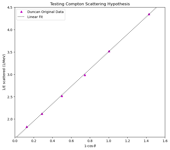
Fig. 9.6 Guilford College student Alison Duncan reproduced Compton’s experiment in 2005. She used a pulse height analyzer to measure the energy of a photon beam from a Cs-137 source, after the photons had been scattered off an aluminum target. The graph uses the same axes as Fig. 9.5.

11. Fig. 9.6 shows some results of a scattering experiment performed by Alison Duncan during the spring semester of 2005 as part of her first year lab. She collimated a beam of photons from a Cs-l37 radioactive source and aimed the beam at an aluminum target. She then used a NaI detector to measure the energy of the photons that were scattered at various angles with respect to the initial beam line. Her plot shows the reciprocal of the measured energy plotted as a function of \((1-\cos{\theta})\) where \(\theta\) is the scattering angle of the photons.

slp = b
icpt = a
E0=1/slp
Eg = 1/icpt
eslp = 0.01209
eicpt = 0.009785
eE0 = eslp*E0**2
eEg = eicpt*Eg**2
print("The best-fit slope is ({0:4.3f} +- {1:4.3f}) 1/MeV".format(slp,eslp))
print("The best-fit y-intercept is ({0:4.3f} +- {1:4.3f}) 1/MeV".format(icpt,eicpt))
print("The estimate of E0 is ({0:4.0f} +- {1:1.0f}) keV".format(E0*1000,eE0*1000))
print("The estimate of Egam is ({0:4.0f} +- {1:1.0f}) keV".format(Eg*1000,eEg*1000))

The best-fit slope is (1.943 +- 0.012) 1/MeV
The best-fit y-intercept is (1.563 +- 0.010) 1/MeV
The estimate of E0 is ( 515 +- 3) keV
The estimate of Egam is ( 640 +- 4) keV

a) Are her data consistent with Compton’s model of photon-electron scattering? Give evidence.

b) Which number reported from the fit estimates the rest energy of the particle off of which the photons scattered? Does this value make sense to you? Why?