11. The Electromagnetic Tensor

Many introductory relativity textbooks stop with dynamics, but I think it’s important to include some of the implications of realtivity theory for the understanding of electricity and magnetism. There are two reasons why it’s important to see how SR affects E&M: first, for mechanics, the effects of relativity are completely negligible in our world of physics professors and dump trucks. The weird effects only show up at speeds near the speed of light, and for most day-to-day processes you can blissfully ignore them.

Within the context of electricity, however, relativistic effects occur, and are important, at any speed. Even for the literal snail’s pace of the average drift speed of a 1 A current in a copper wire, the differing observations in reference frames in relative motion are obvious and unavoidable.

Second, the theory of electrodynamics that culminates in Maxwell’s Equations is automatically consistent with SR. Newtonian mechanics needs massive modifications to work with SR, but the bulk of relativistic E&M is learning how to write it in four-vector notation and remarking, “Wow! It works!” For a full treatment of this topic, I recommend an advanced electrodynamics book such as [Griffiths, 2023]. In this eBook, I only plan to introduce the subject, not explore all the implications.

11.1. Magnetic Force as a Relativistic Effect

11.1.1. Reminder of Classical Situation

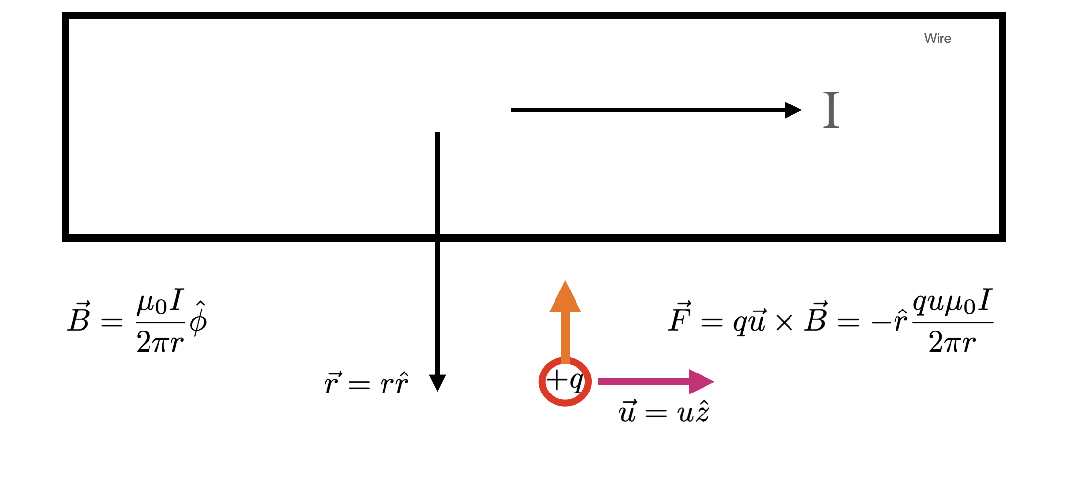
Fig. 11.1 Schematic of the classical understanding of the force on a charge moving antiparallel to a current-carrying wire. A description of all the pieces of this figure is in the text.

Before we dive into tackling how relativity implies we must rethink E&M, let’s first walk through a classical understanding of a simple problem. Then we will recast that problem through a relativistic lens and see how it invites a different understanding of the phenomenon. We will start with the force on an electric charge moving parallel to a current-carrying wire. The situation is shown in Fig. 11.1 as a schematic. A wire carries a current \(I\) to the right. Meanwhile a charge \(q\) is moving to the right with a velocity \(\vec{u}\) at a distance \(r\) from the center of the wire. We observe, empirically, that the charge experiences an upward force (toward the wire) with a magnitude of

(11.1)\[\vec{F} = -\hat{r} \frac{qu\mu_0 I}{2\pi r}\]

and this force remains perpendicular to the motion of the particle, no matter how we rotate the system around the wire.

We therefore invent a field we call \(\vec{B}\) and we say there’s a magnetic force \(\vec{F}_m = q\vec{u}\times\vec{B}\). To make that force line up with the observed force, we say the field \(\vec{B}\) points tangent to a circle around the wire and has a magnitude of \(\mu_0 I/2\pi r\).

11.1.2. The Relativistic Model

As with most relativity problems, this one comes down to setting up the situation in different reference frames and then switching between them with Lorentz transformations. There are three frames we will need to compare, because there are two different kinds of motion (the current and the charge), and we need to compare them both to a common reference frame. Or to put it another way, we have the initial frame in which the charge has a velocity \(\vec{u}\), we have the rest frame of the charge, and then we will need the rest frame of the current, as well.

Let us begin with the “lab frame”, which I will call “Frame A”, which corresponds to the situation described in the previous section. There is a current \(I\) to the right, but I am going to break this down into two parts: a positive current going right and a negative current going left. Each current comprises half the charge density, but they are equal and opposite densities, so the total charge density is zero (which is to say the wire is electrically neutral), but the total current is \(I\) to the right. This way of conceptualizing the setup is shown in Fig. 11.2, with the positive current in red and the negative current in blue.

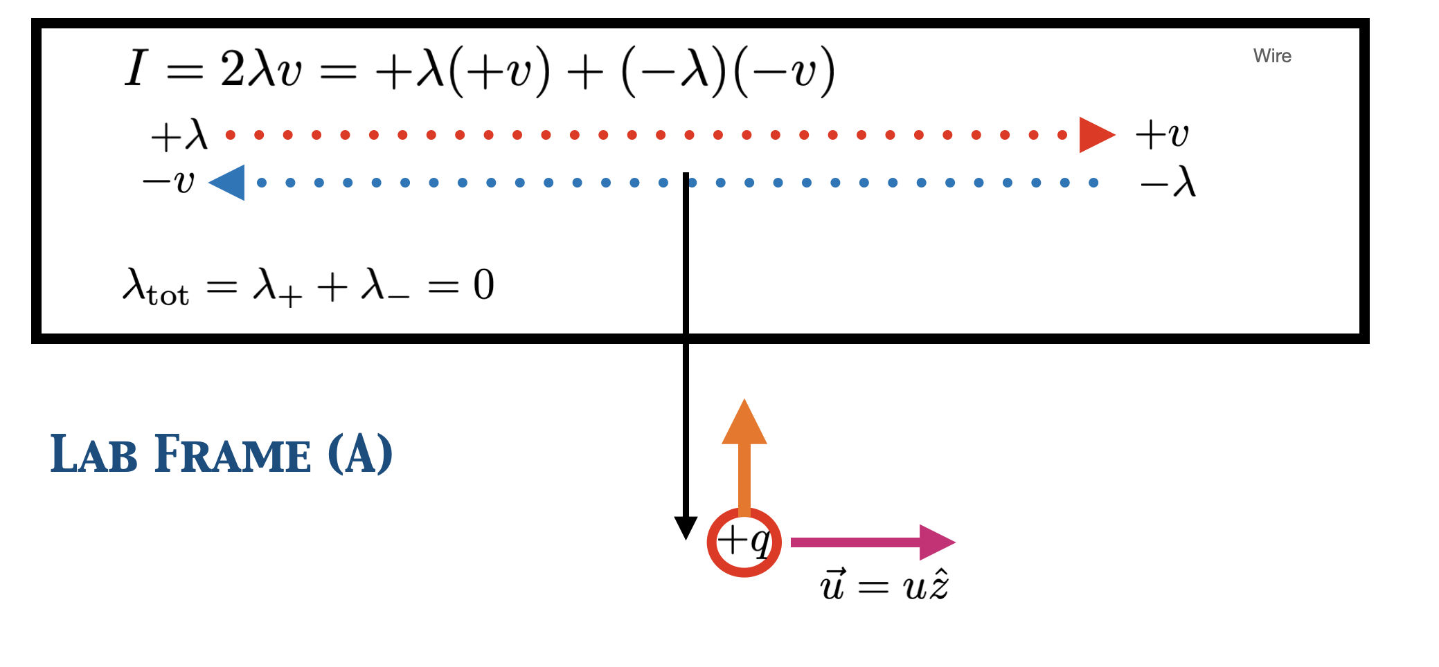
Fig. 11.2 Schematic of a particular way of visualizing the current \(I\) in a reference frame where the total charge density of the wire is zero. We define the current as \(2\lambda v\), but there is a \(+\lambda\) moving to the right (red) and a \(-\lambda\) moving to the left (blue). The sum of the two \(\lambda\) is zero, but since the \(v\) values are also opposite, \(\lambda v\) adds up instead of cancelling.

We then need to transform into a frame moving with \(v_R=u\) to the right. In this frame, which I will call Frame B, the charge \(+q\) is at rest. According to the classic magnetic force model (Equation (11.1)), the magnetic force on the charge should be zero. It is not moving, so it cannot experience a magnetic force. However, since an observer in Frame A observes the charge being attracted to the wire, an observer in Frame B must also observe the charge being attracted to the wire. But how, if there is no force? No magnetic force! There could be a different force.

Note

This is actually the exact sort of dilemma that led Einstein to develop SR in the first place. How could you have a magnetic force in one reference frame, and an electric force in another reference frame? Shouldn’t the laws of Physics be the same in all reference frames? Einstein was troubled by the idea that two different models were needed to describe the same phenomenon, purely dependent on your choice of reference frame. His 1905 paper that introduced SR to the world was not called “Special Relativity” after all. The name of that paper was “On the Electrodynamics of Moving Bodies”.

In Frame B, illustrated in Fig. 11.3, lengths along the direction of relative motion will be contracted. When we talk about a charge density \(\lambda\), we are talking about a certain number of charges per length. So the charge densities in the wire will change, and since these sets of charges have different velocities, relative to \(\vec{v}_R\), they will contract by different amounts. Given our formula for length contraction, we know

(11.2)\[\lambda_\pm =\pm\frac{dq}{dz} = \pm\gamma_\pm\frac{dq}{dz_0} = \pm\gamma_\pm\lambda_0\]

In this frame, the two charge densities will not cancel out, since they will no longer be equal. The wire will not be electrically neutral.

(11.3)\[\lambda_{\rm totB} = \lambda_+-\lambda_- = \lambda_0(\gamma_+-\gamma_-)\]

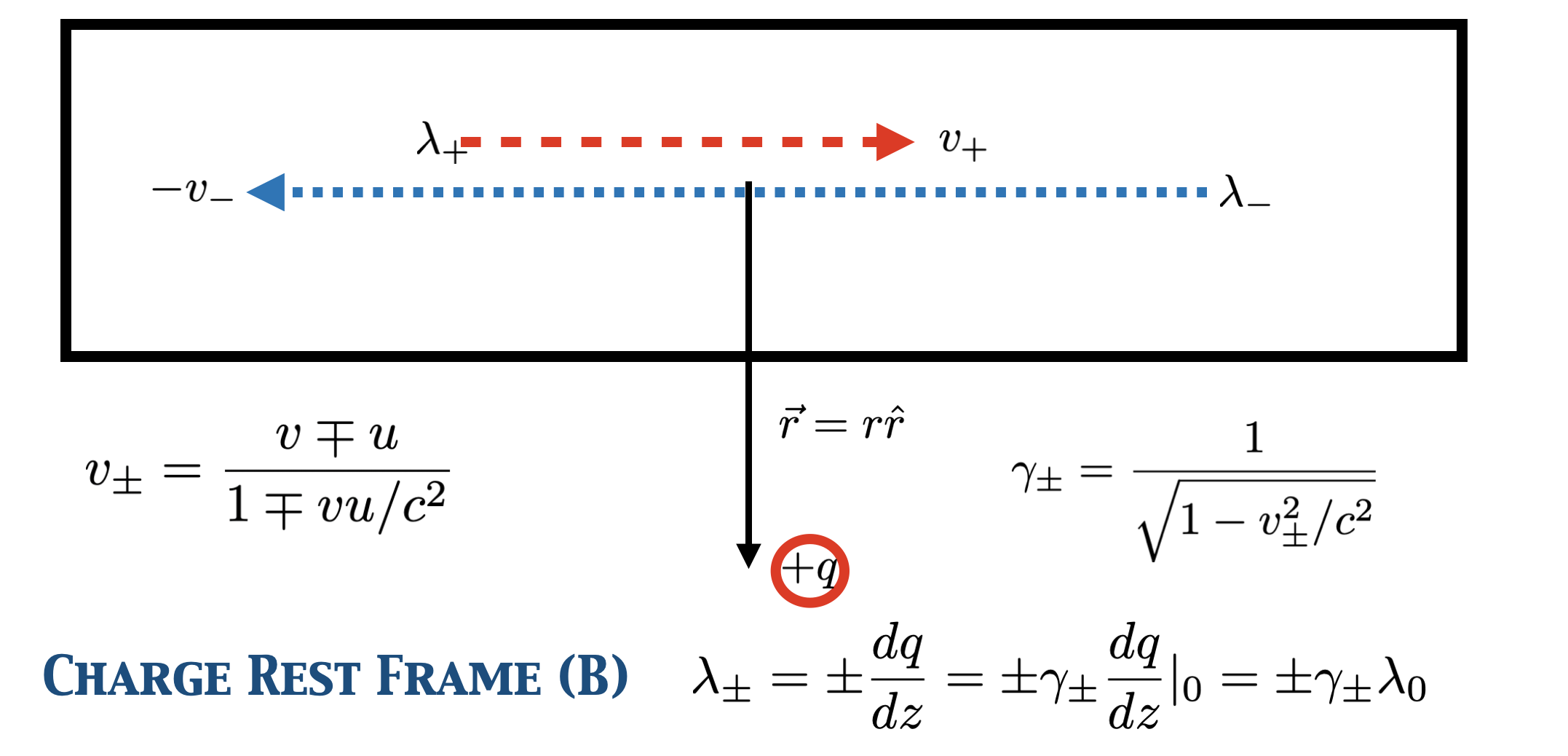
Fig. 11.3 Schematic of a reference frame in which the single charge is at rest and the wire is moving to the left with a speed \(u\). In this frame, because the positive and negative charges are moving at different speeds, the distances between those charges will be contracted by different amounts.

To be more specific, instead of talking about just one \(\lambda\), we must now talk about a \(\lambda_+\) and a \(\lambda_-\), since they will be different. (Note that \(\lambda_\pm\) is explicitly defined in Frame B). To know how much they are contracted, we have to know their speeds. We have a formula for that:

(11.4)\[v_\pm = \frac{v\mp u}{1\mp uv}\]

where \(v\) (the speed of the current) and \(u\) (the relative velocity between A and B) are measured in Frame A. On the other hand,

(11.5)\[\gamma_\pm = \frac{1}{\sqrt{1-v_{\pm}^2/c^2}}\]

where \(v_\pm\) is measured in Frame B.

But what are \(v_\pm\) measured with respect to? These velocities represent the velocities of the charges in the wire, the \(+\) and \(-\) charges separately, but velocity relative to what?

We need a Frame C, in which the positive charges in the wire are at rest. In Frame C, the charge density of the positive charges will be \(\lambda_0\) (we don’t actually need to know what the charge density of the negative charges in Frame C is – we just need an anchor point with which to compare the others). If the positive charges are at rest in Frame C, that means that Frame A is moving with speed \(v\) with respect to Frame C! The original speed of the charges in Frame A was \(v\). So this means that \(\lambda = \gamma\lambda_0\), where \(\gamma=1/\sqrt{1-v^2/c^2}\).

We now have all the pieces we need to pull it all together. To make the math easier to write, I will take \(c=1\) for a while, and then put the \(c\) back later. From comparing Frames A and C, we know \(\lambda = \gamma\lambda_0\), where \(\gamma = 1/\sqrt{1-v^2}\). From comparing Frames B and C, we know \(\lambda_\pm = \pm\gamma_\pm\lambda_0\), where \(\gamma_\pm = 1/\sqrt{1-v_\pm^2}\). We also know that \(v_\pm = (v\mp u)/(1\mp vu)\). If we plug in the velocity formula for \(v_\pm\), we get

(11.6)\[\gamma_\pm = \frac{1}{\sqrt{1-\left(\frac{v\mp u}{1\mp uv}\right)^2}}\]

find a common denominator and flip it upside down to get

(11.7)\[\gamma_\pm = \sqrt{\frac{(1\mp uv)^2}{(1\mp vu)^2 - (v\mp u)^2}}\]

Expand out the squared terms in the denominator

(11.8)\[\gamma_\pm = \frac{1\mp uv}{\sqrt{(1\mp 2vu+v^2u^2 - v^2\pm 2vu-u^2)}}\]

Note the factors of \(2vu\) will cancel, as whatever sign they have, the other will be opposite. That will leave \(1+v^2u^2-v^2-u^2\) in the denominator, but that’s just the same as \((1-v^2)(1-u^2)\) and \(1/\sqrt{1-v^2}\) is just \(\gamma\)! So this becomes

(11.9)\[\gamma_\pm = \gamma\frac{1\mp uv}{\sqrt{(1-u^2)}}\]

Now we have equations for \(\gamma_\pm\), we can figure out the total charge density in Frame B:

(11.10)\[\lambda_{\rm totB} = \lambda_++\lambda_- = \lambda_0(\gamma_+-\gamma_-)= \gamma\lambda_0\left[\frac{1-vu}{\sqrt{1-u^2}}-\frac{1+vu}{\sqrt{1-u^2}}\right] = \lambda\left[\frac{-2vu}{\sqrt{1-u^2}}\right]\]

Note that the total density in Frame B is negative! There are some important pieces in this equation we can pull out. Notice the \(2\lambda v\). This is what we would call \(I\) in the original Frame A. Furthermore \(1/\sqrt{1-u^2}\) is just the \(\gamma_R\) for the transformation between Frames A and B.

We know that a line charge density in Frame B will have an electric field given by

(11.11)\[\vec{E} = \hat{r}\frac{\lambda_{\rm totB}}{2\pi \epsilon_0 r}\]

But we have an equation for \(\lambda_{\rm totB}\), it’s Equation (11.10)!

(11.12)\[\vec{E} = \hat{r}\frac{-Iu}{2\pi \epsilon_0 rc^2}\gamma_R\]

where I put the \(c\) back in, now. Since \(\vec{F}_e = q\vec{E}\), and using \(c^2=1/\mu_0\epsilon_0\), we can write this as

(11.13)\[\vec{F}_E = q\vec{E} = -\hat{r}\frac{qu\mu_0I}{2\pi r}\gamma_R\]

for the electric force experienced in Frame B. If we want to switch back into Frame A, we use the formula we found for the Minkowski force (Equation (10.17)) and drop the \(\gamma_R\) to get

(11.14)\[\vec{F}_{EA} = \vec{F}_{EB}/\gamma_R = -\hat{r}\frac{qu\mu_0I}{2\pi r}\]

This is the exact same force that, classically, we would have said was a magnetic force! We had the same equation back at the start of the chapter, as Equation (11.1)!

Note

You will note that nothing in this analysis requires that any of the speeds, \(u\) or \(v\) or \(v_\pm\), be close to the speed of light. In fact, you may remember from Intro E&M that even a current as large as 1 A in a copper wire only requires an average drift speed of something like \(10^{-4}\) m/s. And yet the moving charge will be deflected, even at small speeds, and so if you want to model that force without introducing magnetism, you must use SR, even with tiny speeds. In mechanics, you generally need to move at speeds near \(c\) to observe the relativistic effects, but for E&M, you need SR at any speed.

So which is it? Magnetic or Electric? The answer is both and neither! We are heading toward an understanding that there is just one “thing” that we currently call an electromagnetic field, and whether we name it “electric” or “magnetic” depends on which reference frame you’re observing in. If SR had been developed before magnetism was discovered, we probably wouldn’t even have a word for “magnetic field” – there would just be result of transforming an electric field into another reference frame. Just like we now talk about “spacetime”, and the space and time parts get mixed up when you change frames, and just like how \(x\) and \(y\) get mixed up when you rotate your coordinates around the \(z\) axis, it seems that \(\vec{E}\) and \(\vec{B}\) get mixed up when you switch reference frames, too.

But we can’t just make a four vector out of them! They have six components, not four. To understand how to fold \(E\) and \(B\) into the SR formalism, we must first figure out how they transform when you switch frames. Then we can see if and how the Lorentz transformation is relevant to them.

11.2. How the Fields Transform

The goal for this section is to develop a model for how electric and magnetic fields will change when we switch to another frame of reference, moving with a velocity \(\beta_R\) along the \(x\) axis. Once we have that set of transformations, we can connect them to the Lorentz transformations we already know, and thereby construct an equation that will let us predict how \(\vec{E}\) and \(\vec{B}\) will change. This will bring electric and magnetic fields into the SR formalism.

The most important concept to remember going into this analysis is that fields are not independently existing entities. Fields are a way of keeping track of where the charges are. You can’t have a field just existing, by itself, with no charges. If you have a field here, there must be charges somewhere that are causing that field. If you can figure out what happens to the charges, you can figure out how the fields will change.

The second thing you need to remember is that all the rules for figuring out fields, like calculating the flux through a Gaussian surface and connecting that to the charge inside, or calculating the line integral of an Amperian loop and connecting that to the current flowing through the loop – all those rules still work in any reference frame. Remember the first postulate: the laws of physics will be the same in any reference frame.

With this in mind, we can start constructing rules for how to get the fields in a relatively moving reference frame, if we know the situation in different reference frame. Let’s start with the simplest situation: a uniform electric field in the \(x\) direction. What kind of charge distribution will give us a uniform \(\vec{E}\) in the \(x\) direction? Well, set up a parallel plate capacitor such that the plates are parallel to the \(yz\) plane, and you will get a roughly uniform field between the plates, perpendicular to them, which is indeed the \(x\) direction. The magnitude of the field is the charge density on the plates divided by \(\epsilon_0\).

How will this situation change if we switch into a passing reference frame? Well, any time interval would dilate, but this is a static situation, so there are no relevant time intervals. Any length along the direction of the relative velocity will contract, so the distance between the plates will get smaller, but the value of the field does not depend on the distance between the plates. The density of charge on the plates will not change, so the field will not change. Therefore

(11.15)\[\boxed{ E'_x = E_x }\]

How about a uniform magnetic field? The way to get a uniform magnetic field is to have a current-carrying solenoid. Then you will get a nearly uniform field inside the coil with a value of \(\mu_0 n I\), pointed along the axis of the solenoid, where \(n\) is the number of coils per length. Orient the solenoid so that the axis of the coil is along the \(x\) axis. Now when we switch to a passing reference frame, the length along the axis of the coil will contract! So the number of coils per length will increase: \(n' = \gamma n\). So you might think the magnetic field will increase. But wait! This situation is not static! There is a current moving, and current is \(dq/dt\), so there is also a relevant time interval, which will dilate by the same factor \(\gamma\)! So the current will go down by the same factor that the coil density goes up, the two factors of \(\gamma\) will cancel each other out, and the magnetic field will remain unchanged:

(11.16)\[\boxed{ B'_x = B_x }\]

Fig. 11.4 Animation of how the current and \(B\) field of a solenoid are affected by changing into a different reference frame. The red dots represent charges moving around a cylindrical solenoid. One row of them is turned white purely to help you see how fast they are going around. The blue arrows show representative \(B\) field vectors inside the solenoid. The slider allows you to change the relative velocity between the reference frames. The magenta arrow shows the velocity of the cylinder in that frame. The animation cheats, though, by not showing the cylinder in motion (it would be frustrating to have to chase after it). The circles will compress due to length contraction, but the rate of rotation (the current) will slow due to time dilation. These effects cancel, leaving the \(B\) field unchanged.

Now things get a little more complicated. If we want to get the \(E\) field components in the perpendicular directions, we can keep the same parallel plate capacitor, but we have to rotate it so that the \(E\) field now points, say, up along the \(y\) axis. The plates of the capacitor are now parallel to the \(xz\) plane. When we switch into another reference frame, the dimension that contracts is along one dimension of the plates, so the charge density will increase: \(\sigma' = \gamma \sigma\). This means the magnitude of \(E_y\) will also increase to \(\gamma E_y\).

But wait! In this new primed reference frame, the plates will be moving in the \(-x\) direction! That means in this reference frame, there will be a current that wasn’t there in the unprimed frame, and that means there will be a \(B\) field in this reference frame that wasn’t there in the unprimed frame! If you draw a square Amperian loop with side \(L\), lying in the \(yz\) plane, and place it so that one side of it runs along the \(z\) axis and the opposite side is outside the capacitor, then there will be a current of \(\sigma' v_R L\) that runs through that square. The loop integral around that square will be \(B_z L\), so there will be a magentic field of \(\mu_0 \sigma' v_R\) in the \(-z\) direction. We can write this in terms of the original unprimed variables by putting in a \(\gamma\): \(B'_z = -\mu_0 \gamma \sigma v_R\). An interactive animation of this situation is shown in Fig. 11.5, where you can change the relative velocity of the frames and see how the fields change.

Fig. 11.5 Animation of how the charges and fields are affected by changing into a different reference frame. The orange dots represent charges spread over a plate of a parallel plate capacitor (the opposite plate is not shown). The slider and the magenta arrow are the same as in Fig. 11.4. Also as in Fig. 11.4, the actual motion of the plate along \(x\) is not shown. The dots will compress due to length contraction. The cyan arrows show the electric field, while the white arrows show the magnetic field. The red-green-blue arrows at the center show the x-y-z cartesian axes, in that order.

This means we really picked a special case when we first chose our rotated capacitor at rest – we chose the only frame where \(B_z = 0\). To get a general rule for how \(E\) and \(B\) transform, we should have chosen a frame in which the capacitor was already moving, and then transformed into a frame where the capacitor is moving at a different speed. Then we will have a general rule for how \(E_y\) and \(B_z\) transform. So let’s consider the primed frame we just derived as the unprimed frame, and transfer to a different primed frame. Let \(v_R\) be the relative velocity between these two frames, and say the unprimed frame is moving with a velocity \(u\), relative to the frame where the capacitor is at rest (which means there is a Lorentz factor of \(\gamma_u=1/\sqrt{1-u^2/c^2}\) between the unprimed frame and the rest frame). In that case, the fields in the unprimed frame will be

(11.17)\[\vec{E} = \gamma_u \sigma_0 /\epsilon_0\hat{y}\]

and

(11.18)\[\vec{B} = \mu_0 \gamma_u \sigma_0 u \hat{z}\]

We now want to switch into a reference frame that is moving at \(v_R\) relative to this new unprimed frame. We will also need to relate the primed reference frame back to the rest frame, so note that

(11.19)\[v' = \frac{v_R+u}{1+v_Ru/c^2}\]

is the speed of the primed frame relative to the rest frame, and we will need a \(\gamma' = 1/\sqrt{1-v'^2/c^2}\). This means that the charge density on the plates will be \(\sigma' = \gamma'\sigma_0\) in the new primed frame. If we were an observer living in this new primed frame, we would say there was an electric field of \(\vec{E}' = \hat{y}\sigma'/\epsilon_0\) and a magnetic field of \(\vec{B}' = -\hat{z}\mu_0 \sigma' v'\). Our goal is to write these field equations, as defined in the primed frame, in terms of the quantities an observer in the unprimed frame would measure.

Let’s look at the electric field first. We know that the charge density in the unprimed frame is \(\sigma = \gamma_u \sigma_0\). And we know \(\sigma' = \gamma' \sigma_0\). Therefore, \(\sigma' = \sigma \gamma'/\gamma_u\). We can (with some effort) simplify that ratio of Lorentz factors (I am going to use \(c=1\) and then put the \(c\) back at the end):

(11.20)\[\frac{\gamma'}{\gamma_u} = \sqrt{\frac{1-u^2}{1-v'^2}} = \sqrt{\frac{1-u^2}{1-\left(\frac{v_R+u}{1+v_Ru}\right)^2}} = \sqrt{\frac{(1-u^2)(1+v_Ru)^2}{(1+v_Ru)^2-(v_R+u)^2}}\]

Expand the denominator and take the square root of the square in the numerator:

(11.21)\[\frac{\gamma'}{\gamma_u} = (1+v_Ru)\sqrt{\frac{1-u^2}{1+2v_Ru+v_R^2u^2-v_R^2-2v_Ru-u^2}}\]

Cancel out the common factors in the denominator:

(11.22)\[\frac{\gamma'}{\gamma_u} = (1+v_Ru)\sqrt{\frac{1-u^2}{1+v_R^2u^2-v_R^2-u^2}}\]

The four terms in the denominator are just \((1-v_R^2)(1-u^2)\), and the factor of \((1-u^2)\) will cancel! That leaves (putting the \(c\)s back)

(11.23)\[\frac{\gamma'}{\gamma_u} = \frac{1+v_Ru/c^2}{\sqrt{1-v_R^2/c^2}} = \gamma_R(1+v_Ru/c^2)\]

This means we can write our primed electric field as

(11.24)\[E'_y = \frac{\sigma}{\epsilon_0} \gamma_R(1+v_Ru/c^2)\]

but \(1/c^2=\mu_0\epsilon_0\), so if we multiply through the parentheses, we get

(11.25)\[E'_y = \gamma_R \frac{\sigma}{\epsilon_0} + \gamma_Rv_R\mu_0 \sigma u\]

But those equations contain the formulae for \(E_y\) and \(B_z\) in the unprimed frame! So we end up with

(11.26)\[\boxed{ E'_y = \gamma_R E_y - \gamma_Rv_RB_z }\]

So, much like we talked about with rotations, the electric and magnetic fields are getting mixed up when you switch reference frames. Also similar to the force on a charge moving next to a current, what looks like \(E\) in one frame has \(E\) and \(B\) mixed together in another frame.

We can follow a similar process with \(B'_z\):

\[B'_z = -\mu_0 \sigma' v' = -\mu_0 \sigma \frac{\gamma'}{\gamma_u} \frac{v_R+u}{1+v_Ru/c^2} = -\mu_0 \sigma \gamma_R(1+v_Ru/c^2) \frac{v_R+u}{1+v_Ru/c^2}\]

using Equation (11.23) to get rid of the ratios of gammas. There is a common factor in both numerator and denominator that will cancel!

(11.27)\[B'_z = -\mu_0 \sigma v_R \gamma_R - \mu_0\sigma\gamma_R u \]

The second term is just the original \(B_z\) times a \(\gamma_R\) factor, and the first term depends on \(\sigma\), which we know is proportional to the original \(E_y\), so we can plug in the formulae for the fields to get

(11.28)\[\boxed{ B'_z = \gamma_R B_z - \gamma_R \frac{v_R}{c^2}E_y }\]

To make sure you have understood the logic, here, you should rotate the capacitor and work out the last two components yourself. If you rotate the capacitor so that the plates lie parallel to the \(xy\) plane, then you’ll get \(E_z\), and the motion of the capacitor in \(x\) will make a magnetic field in the \(+B_y\) direction. Once you convince yourself of that, the rest of the math is exactly the same, just substituting \(E_z\) for \(E_y\) and \(+B_y\) for \(-B_z\). You should get

(11.29)\[\boxed{ E'_z = \gamma_R E_z + \gamma_Rv_RB_y }\]

and

(11.30)\[\boxed{ B'_y = \gamma_R B_y + \gamma_R \frac{v_R}{c^2}E_z }\]

All right, that tells us how all three components of \(\vec{E}\) and \(\vec{B}\) will change when you switch to a relatively moving reference frame. Now what do we do with them, and how does this relate to the Lorentz transformation we have used for such a change up to this point?

11.3. A paradox that shows why the fields must change

Let’s think through a possible experiment that one could (in principle) do that would reveal why \(E\) and \(B\) have to transform like this. A full solution of this problem is beyond the scope of this course, but we can work through the problem at a conceptual level.

You will have learned that a charged particle like an electron in the presence of a magnetic field will move in a circle perpendicular to the field. The faster it goes, the wider the circle, and the stronger the field, the smaller the circle. Consider a cart that is carrying an apparatus, like a solenoid or a Helmholtz coil, that can make a vertical magentic field. An electron travels horizontally into the field region, and will start flying in a horizontal circle. There is no electric field in this reference frame. All seems well (ignoring gravity, of course).

However, what if we start pushing the cart at a very slow speed (nm/s, if you like. Really slow.) along the ground. If you didn’t know relativity, you would think, there’s no reason for the electron to change its motion. The field is uniform, the electron just keeps going in a circle – what the cart does has nothing to do with it. So you would expect the cart to just move slowly along until it moves out from under the electron, at which point the electron is outside the field, and it will shoot off into space.

However, now consider this situation from the reference frame where the cart is at rest and the lab is moving. According to our postulates, if the cart moves out from under the electron in the rest frame of the lab, the electron would have to drift off the cart (in the opposite direction) in the rest frame of the cart. However, in the cart frame, nothing relevant is moving – it’s exactly the same as the original lab frame when the cart was at rest. So there is absolutely no reason why the electron would start drifting off the cart at all, and the symmetry is such that there’s no reason for the electron to pick the direction of the lab motion for its drift direction, if it were to drift, which it wouldn’t. There is no reason for the electron to move in any particular direction except around in its circle.

What is the resolution of this paradox? Now that you know how the \(E\) and \(B\) fields transform, you will understand that when you switch reference frames from the frame where the cart is at rest (vertical \(\vec{B} = B_y\hat{y}\), \(E=0\)) to a frame where the cart is moving, there will be an electric field in the \(z\) direction in the new frame (\(E'_z = \gamma_Rv_RBy\)), in addition to the altered value of \(B\) (\(B'_y = \gamma_R B_y\)). Although solving the equations of motion under these primed fields is beyond the scope of this book, the solution is a shape much like the path of a point on the wheel of a bicycle – the center of the circular motion will move in the \(+x\) direction at the speed of the cart. This trajectory is shown in Fig. 11.6, and an animation is shown in Fig. 11.7. The electron will not fall off the edge of the cart in either frame: the center of its circular motion is at rest with respect to the cart! If the cart is moving, so does the center of the circle. The electron stays with the cart.

You can’t resolve this paradox without relativity, and the speeds involved are obviously nowhere even close to the speed of light.

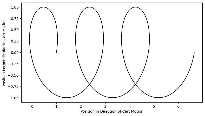
Fig. 11.6 Plot of electron trajectory in frame with moving cart. The center of the circle drifts right with the same speed as the cart. If you were to transform this shape back into a frame moving at \(+v\), the trajectory would be a circle, and the cart would be at rest.

Fig. 11.7 Animation of how the cyclotron motion of an electron in a magnetic field changes in reference frames in relative motion. The red sphere is an electron, and the orange rectangle is the cart described in the text. The translucent square represents a region of magnetic field. Buttons will show or hide magnetic (blue) and electric (yellow) field vector arrows, as well as the total force on the electron (green). First, leave the speed at zero and click the button to run the animation in the rest frame of the cart. Rotate the perspective to see the circular cyclotron motion from above. Unclick the button to stop the animation, then move the slider. Now when you click the button, the cart will move, but there will be an electric field as well as the magnetic field. Again, if you rotate the display and view from above, you can see how the force on the electron changes to keep the electron with the cart as it moves. Try some different speeds!

11.4. The Electromagnetic Field Tensor

For the rest of this book up to this point, when we wanted to see what would happen to some quantity when measured in a reference frame in relative motion, we cast the quantity in question as a four-vector and performed a Lorentz transformation. We can’t do that, here, because \(\vec{E}\) and \(\vec{B}\) together have six components, which don’t easily fit into a four-vector. We need some way to deal with these fields, and we need to use the Lorentz transformation, because the success of all those four vectors shows us that the Lorentz matrix is indeed the correct way to switch reference frames.

Before we start working toward a solution, let me copy all the relevant equations here so we have them in one place:

\[E'_x = E_x\hspace{3cm}B'_x = B_x\]

\[E'_y = \gamma_R E_y - \gamma_Rv_RB_z\hspace{3cm} B'_y = \gamma_R B_y + \gamma_R \frac{v_R}{c^2}E_z\]

\[E'_z = \gamma_R E_z + \gamma_Rv_RB_y\hspace{3cm} B'_z = \gamma_R B_z - \gamma_R \frac{v_R}{c^2}E_y\]

and recall that the Lorentz matrix can be written as

(11.31)\[\begin{split}\Lambda^\alpha_\beta = \begin{pmatrix} \gamma_R & -\gamma_R\beta_R & 0 & 0\\ -\gamma_R\beta_R & \gamma_R & 0 & 0\\ 0 & 0 & 1 & 0\\ 0 & 0 & 0 & 1 \end{pmatrix}\end{split}\]

Note now I have switched to using Einstein notation and have left out the complex number \(i\). The letter \(\alpha\) refers to the row number of the matrix, and the \(\beta\) refers to the column number (0 through 3, of course). So \(\Lambda^0_1 = -\gamma_R\beta_R\) (first row, second column). Of course, this is also the same number as \(\Lambda^1_0\) – with the complex number notation, these numbers had opposite sign, to account for the \(i^2\), but that is not necessary in this notation.

Note

At this point, you may wish to go back to Chapter 3 and re-read the section on Einstein notation.

At this point, many books jump to the answer and show that it works. While there is nothing formally wrong with that, it’s not very emotionally satisfying. I’d like to give you some kind of intuition as to why you might want to make that jump, rather than just tell you the answer. In no way is what I am about to do any kind of derivation; what I want to do is give you a kind of guide to get you to the answer, not a proof.

We have six numbers (two vectors) and a \(4\times 4\) matrix that we think must be involved with the transfer somehow. If there were a simple way to put each three vector into a four-vector, you might think that maybe the thing to do would be to perform two Lorentz transformations: one for \(E\) and one for \(B\). However, we need to make the dimensions match up. You can’t multiply a \(4\times 4\) matrix by a three-row column.

If it were as simple as performing two Lorentz transformations, you would write that as

(11.32)\[\Lambda^\alpha_\beta\Lambda^\mu_\nu\]

where the \(\alpha\) and \(\mu\) refer to the rows and the \(\beta\) and \(\nu\) refer to the columns.

This short equation represents multiplying two \(4\times 4\) matrices together. That’s going across each row and down each column 16 times, and what you end up with is another \(4\times 4\) matrix. But that gives a clue. Maybe what we need to do is fit the six field components into a \(4\times 4\) matrix somehow. If we could do that, then we could multiply these two Lorentz matrices by that field matrix, and the result would be another \(4\times 4\) matrix, which we could interpret as the values of the same matrix, just in the new relative reference frame. Mathematically, that would be

(11.33)\[F'^{\alpha\mu} = \Lambda^\alpha_\beta\Lambda^\mu_\nu F^{\beta\nu}\]

The Einstein notation means that this equation is really representing sixteen equations, one for each term in the \(4\times 4\) matrix that results from all these multiplications. There’s a double sum over \(\beta\) and \(\nu\), leaving single values for \(\alpha\) and \(\mu\) unchanged from the right side to the left. So a single one of these sixteen terms would look like

(11.34)\[\begin{split}F'^{01} = \Lambda^0_0\Lambda^1_0 F^{00} + \Lambda^0_0\Lambda^1_1 F^{01} + \Lambda^0_0\Lambda^1_2 F^{02} + \Lambda^0_0\Lambda^1_3 F^{03} +\\ \Lambda^0_1\Lambda^1_0 F^{10} + \Lambda^0_1\Lambda^1_1 F^{11} + \Lambda^0_1\Lambda^1_2 F^{12} + \Lambda^0_1\Lambda^1_3 F^{13} +\\ \Lambda^0_2\Lambda^1_0 F^{20} + \Lambda^0_2\Lambda^1_1 F^{21} + \Lambda^0_2\Lambda^1_2 F^{22} + \Lambda^0_2\Lambda^1_3 F^{23} +\\ \Lambda^0_3\Lambda^1_0 F^{30} + \Lambda^0_3\Lambda^1_1 F^{31} + \Lambda^0_3\Lambda^1_2 F^{32} + \Lambda^0_3\Lambda^1_3 F^{33}\end{split}\]

You have to think about Einstein notation like writing a computer program: once you assign \(\alpha\) a particular value, like \(0\), then that value has to go in everywhere that there’s an \(\alpha\). So you can see in Equation (11.34) that there’s a \(1\) in the \(\mu\) location, so everywhere in the huge sum where there would be a \(\mu\), there’s a \(1\) in each of those locations (the superscript on the second \(\Lambda\)). The lower index on the second \(\Lambda\) is always the second number in the superscript on the \(F\), because those positions both have a \(\nu\) in Equation (11.33).

Now, this looks like a huge mess, but luckily for us, most of the numbers in the \(\Lambda\) matrix (Equation (11.31)) are zero! All the examples of \(\Lambda\) elements in the specific case of Equation (11.34) are either in the first or second row. And the last two columns are both zeros! If we plug in for the elements of \(\Lambda\), we get

(11.35)\[F'^{01} = -\gamma_R^2\beta_R F^{00} + \gamma_R^2 F^{01} + \beta_R^2\gamma_R^2 F^{10} -\gamma_R^2\beta_R F^{11} \]

Now, this looks a bit simpler. The next clue is the fact that there’s a \(\gamma_R^2 + \gamma_R^2\beta_R^2\) in there. If it were just \(\gamma_R^2 - \gamma_R^2\beta_R^2\), that would just be ONE!!! So, what if (crazy thought), what if \(F^{01}=-F^{10}\)? Then the \(\gamma\) and \(\beta\) factors would disappear, and we’d just have \(F^{01}\) in there.

(11.36)\[F'^{01} = F^{01} -\gamma_R^2\beta_R (F^{00} + F^{11} )\]

Now, we know that \(E'_x=E_x\), so this is starting to look like that. What do with the last part, though? Well, if \(F^{01}=-F^{10}\), that suggests that \(F^{00}=0\), as that’s an example of something that is equal to negative itself. If the diagonal elements are all zero, and the matrix as a whole is anti-symmetric, then our specific example of Equation (11.34) has just turned into \(E'_x = E_x\)! Not only that, but if the matrix is indeed anti-symmetric, then instead of sixteen elements, you can discount the diagonal (because those four are all zeros), which leaves twelve, and if half of them are equal and opposite to the other half, we actually only have (drumroll) SIX!!!

We are trying to find a way to use six components of \(\vec{E}\) and \(\vec{B}\), and we already showed that one of the elements of \(F^{\alpha\mu}\) could well be \(E_x\), which suggests that the other five remaining components of \(F^{\alpha\mu}\) could well be the other five components of \(\vec{E}\) and \(\vec{B}\).

So let’s go back to Equation (11.34) and rewrite it to allow for an anti-symmetric matrix:

(11.37)\[\begin{split}F'^{\alpha\mu} = (\Lambda^\alpha_0\Lambda^\mu_1 -\Lambda^\alpha_1\Lambda^\mu_0) F^{01}+ (\Lambda^\alpha_0\Lambda^\mu_2 -\Lambda^\alpha_2\Lambda^\mu_0) F^{02} +\\ (\Lambda^\alpha_0\Lambda^\mu_3 -\Lambda^\alpha_3\Lambda^\mu_0) F^{03} + (\Lambda^\alpha_1\Lambda^\mu_2 -\Lambda^\alpha_2\Lambda^\mu_1) F^{12} +\\ (\Lambda^\alpha_1\Lambda^\mu_3 -\Lambda^\alpha_3\Lambda^\mu_1) F^{13} + (\Lambda^\alpha_2\Lambda^\mu_3 -\Lambda^\alpha_3\Lambda^\mu_2) F^{23} \end{split}\]

Let’s look at another example. What about first row, third column? If \(F^{01}\) might be \(E_x\), maybe \(F^{02}\) is \(E_y\), and we know what that is supposed to be. So let’s look at \(F'^{02}\):

(11.38)\[\begin{split}F'^{02} = (\Lambda^0_0\Lambda^2_1 -\Lambda^0_1\Lambda^2_0) F^{01}+ (\Lambda^0_0\Lambda^2_2 -\Lambda^0_2\Lambda^2_0) F^{02} +\\ (\Lambda^0_0\Lambda^2_3 -\Lambda^0_3\Lambda^2_0) F^{03} + (\Lambda^0_1\Lambda^2_2 -\Lambda^0_2\Lambda^2_1) F^{12} +\\ (\Lambda^0_1\Lambda^2_3 -\Lambda^0_3\Lambda^2_1) F^{13} + (\Lambda^0_2\Lambda^2_3 -\Lambda^0_3\Lambda^2_2) F^{23} \end{split}\]

Now let’s plug in the values of the Lorentz matrices. Anything with a 2 or 3 will be zero, unless it’s a 22 or 33, in which case it’s 1.

(11.39)\[\begin{split}F'^{02} = (\gamma_R \times 0 + \beta_R \gamma_R \times 0) F^{01}+ (\gamma_R \times 1 - 0 \times 0) F^{02} +\\ (1 \times 0 - 0 \times 0) F^{03} + (-\gamma_R\beta_R\times 1 - 0 \times 0) F^{12} +\\ (-\gamma_R\beta_R\times 0 - 0\times 0) F^{13} + (0\times 0 - 0\times 1) F^{23} \end{split}\]

(11.40)\[F'^{02} = \gamma_R F^{02} -\gamma_R\beta_R F^{12}\]

If you compare this result with Equation (11.26), that suggests I can make this work if \(F^{02}\) is \(E_y/c\) and \(F^{12} = B_z\). I need to divide \(E_y\) by \(c\) so that I can multiply the whole equation through by \(c\) and turn the \(\beta_R\) into a \(v_R\) to match Equation (11.26).

Note

But wait, you might say, you said \(F^{01}\) was just \(E_x\)! What’s up with this divide by \(c\) thing? Well, note that if I can say \(E'_x=E_x\), I can also say \(E'_x/c=E_x/c\). That’s just as good. Also, I need all the elements of \(F^{\alpha\mu}\) to have the same dimensions, and to get \(E\) and \(B\) to have the same dimensions, I need to multiply \(B\) times a speed or divide \(E\) by a speed. In principle, you could do it either way, but most people use \(E/c\) rather than \(cB\). Of course, if you use units where \(c=1\), then the question of where to put the \(c\) becomes irrelevant.

You can go through all four remaining elements of \(F^{\alpha\mu}\) and figure out that one way of writing \(F\) that will satisfy Equation (11.33) is:

(11.41)\[\begin{split}\boxed{ F^{\alpha\mu} = \begin{pmatrix} 0 & E_x/c & E_y/c & E_z/c\\ -E_x/c & 0 & B_z & -B_y\\ -E_y/c & -B_z & 0 & B_x\\ -E_z/c & B_y & -B_x & 0 \end{pmatrix} }\end{split}\]

You can (and should) check that you will reproduce the the other four of the six transform equations summarized at the top of this section if you plug this matrix into Equation (11.33). This object is called “the electromagnetic field tensor”, and it combines both \(\vec{E}\) and \(\vec{B}\) into a single object, much like how \(d\vec{x}\) combines \(dx\), \(dy\), and \(dz\) into a single object.

Now, I pulled a fast one on you. When I hit Equation (11.36), I said “well, gosh, we want \(E_x\) to stay the same, so this might be \(E_x\)!”. But if you were paying attention, you might have noticed that the entire sequence of logic following that point could flow just as well if we started from \(B'_x=B_x\) instead of going to \(E_x\) first! If you start with \(B_x\), you would construct the following matrix:

(11.42)\[\begin{split}\boxed{ G^{\alpha\mu} = \begin{pmatrix} 0 & B_x & B_y & B_z\\ -B_x & 0 & -E_z/c & E_y/c\\ -B_y & E_z/c & 0 & -E_x/c\\ -B_z & -E_y/c & E_x/c & 0 \end{pmatrix} }\end{split}\]

This is called the “dual tensor”, and it works just as well as the “regular” EM field tensor. It’s purely a matter of convention that we tend to use the \(F\) rather than the \(G\). They both transform the same way when you switch reference frames. You will see both of these again in the next chapter.

Fig. 11.8 Illustration of how the EM field tensor (displayed to the upper right) relates to the electric and magnetic field vectors (shown as magenta and cyan arrows, respectively). There is a slider for each vector component below the image, and as you change each component, the relevant elements of the EM tensor will change, as will the arrow representation of the vector. Note where the minus signs go. (The value of \(c\) is \(1\), so the units identical for all components.)

11.5. Summary

You have seen in this chapter that it is possible to think of magnetism as simply a manifestation of how space and time distort when you switch into different reference frames. Since all magnetic fields are a mechanism of keeping track of moving charges, just as electric fields are a way of keeping track of charges’ locations, motion is an intrinsic part of what we think of as magnetism, and therefore relativity theory is critically important to understand what’s going on.

Furthermore, we made no assumptions whatsoever about how big the speeds involved are. For mechanics, you don’t need to worry about relativity, but with E&M, there is no such restriction. The effects of Lorentz transformations show up at any speeds.

This in turn suggests that what we call “electric” fields and what we call “magnetic” fields are not independent, separate concepts. By switching reference frames, they get “mixed up”, just like space and time do when you change reference frames. The components of what we call \(\vec{E}\) and \(\vec{B}\) are just whatever numbers fall into the appropriate slots of \(F^{\alpha\mu}\) or \(G^{\alpha\mu}\). Nature does not make a distinction between the two – it’s our own interpretation of the application. There is only one thing that is better called “elecromagnetic field tensor”, much like there is only one thing that we call “spacetime”. The perception that these are separate things are an artefact of the limits of human senses, and it took the hard work and genius of people like Einstein, Lorentz, Minkowski, and others to climb outside those limitations and perceive how the universe works on its own.

11.6. Problems

1. Consider a long line of charge lying at rest along the \(x\)-axis. Say that a little piece of it \(dx\) has a charge \(q=\lambda dx\), where \(\lambda\) is the linear charge density. The electric field in the \(yz\) plane of a piece of line charge at the origin would be

(11.43)\[d\vec{E} = \frac{dx \lambda}{4\pi\epsilon_0(y^2+z^2)^{3/2}}(y\cos{\theta}\hat{y} -z\sin{\theta}\hat{z})\]

(note the full electric field would be an integral over the whole line, but you don’t have to do that for this problem.) The angle \(\theta\) increases counter-clockwise from the \(y\) axis around the \(yz\) plane.

a) Write out the EM field tensor for this situation.

b) Carry out a double-Lorentz transformation (Equation (11.37)) on this tensor to derive the fields from this piece of charge in a frame that is moving with a velocity \(\beta \hat{x}\) relative to the rest frame.

c) Compare your answer with the Biot-Savart Law.

2. Show that the dual tensor \(G^{\mu\nu}\) yields the same transformation rules (e.g. Equation (11.26) or (11.28)) as the field tensor \(F^{\mu\nu}\).

3. Verify that rotating the capacitor as described in the text will indeed produce Equations (11.29) and (11.30).

4. Verify that \(\Lambda^\mu_\nu dx^\nu\) (without the \(i\)) leads to the same transformation equations as \({\cal L}_x(\beta_R)[dx_4]\) did with the \(i\).

5. A velocity filter is a setup that creates crossed \(\vec{E}\) and \(\vec{B}\) fields such that a charged particle moving with the right velocity \(\vec{v} = v\hat{x}\) experiences no net force and will continue moving in a straight line. Assume \(\vec{E}\) is in the \(\hat{y}\) direction and \(\vec{B}\) is in the \(\hat{z}\) direction. Particles that have any other velocity will experience a transverse force and will therefore be pushed out of the beam.

a) What relationship between \(E\) and \(B\) will result in \(\vec{F} = q\vec{E} + q\vec{v}\times\vec{B} = 0\)? (you can guess this from dimensional analysis, but it’s easy enough to solve).

b) Derive the fields in the rest frame of a particle that has this velocity and show that the force on the particle in this frame is still zero.

6. Show that if \(\vec{B}=0\) in the original frame, then in the transformed frame \(\vec{B}' = -(\vec{v}\times\vec{E})/c^2\) and if \(\vec{E}=0\) in the original frame, then \(\vec{E}' = \vec{v}\times\vec{B}\). Compare the last equation to the Lorentz force.

7. What is \(F^{\mu\nu}G_{\mu\nu}\)?