3. Four Vectors

3.1. Time as a Dimension

At the end of the last chapter, we argued that if the speed of light was to be invariant – to be measured the same in any reference frame – then the quantity

\[dx^2 + dy^2 + dz^2 - c^2dt^2\]

must also be invariant across reference frames. This formulation looks a lot like a kind of 4 dimensional Pythagorean theorem, except for the minus sign in the last term. If it were not for that minus sign, we could well imagine we were looking at the magnitude of a four-dimensional displacment vector, just adding time as a new component. If a spacial displacement vector is \(d\vec{r} = (dx,dy,dz)\), and its magnitude squared is \(dx^2+dy^2+dz^2\), perhaps it would make sense to have a four-dimensional vector \(dx_4 = (cdt,dx,dy,dz)\). The problem is that when we square each term of this vector and add them up, we get \(+c^2dt^2\), not minus.

Note

Once you have a displacement \(dx\) and a duration \(dt\), it is possible to define an average veclocity \(v=dx/dt\). Because in Relativity so much is compared to the speed of light, it is useful to express velocities as a fraction of the speed of light. We typically use the greek letter \(\beta\) to represent this fraction. We would say if the velocity were \(2\times10^8\) m/s, that would be two-thirds the speed of light, or \(\beta = 2/3\). Using \(\beta = v/c\) is much more useful than just \(v\) in most cases. Since \(v=dx/dt\), then \(\beta=v/c=dx/cdt\). It would be helpful for you to memorize this now.

We need a way to remember to include that minus sign. There are two ways of keeping track of it. One is simpler for the beginner, and the other makes the more complicated material later easier to manage. First, we look at using the imaginary number \(i^2=-1\) to keep track of the minus sign, and then we will look at the Einstein notation method.

3.1.1. Using Imaginary Numbers

The method that beginners usually find simpler is to introduce complex numbers as a bookkeeping trick. If \(i^2 = -1\), then we can write the time component of the vector as \(icdt\), and its square will be \(-c^2dt^2\). This method ensures that the minus sign always goes in the right place. There is nothing physical or mysterious about the \(i\); it is no more and no less than a handy way to keep track of where to put the minus sign. It always shows up in the time component of the four-vector, and it never shows up in the space components.

Warning

If you ever see a time component without an \(i\), or find an \(i\) in a space component, then you have made a mistake in your math somewhere.

With this tool, we can define a displacement four-vector as

(3.1)\[\begin{split}[dx_4] = \begin{bmatrix} icdt\\ dx\\ dy\\ dz \end{bmatrix}\end{split}\]

Example 3.1

An observer sees two events occuring. She measures a physical displacement of \(dx = 1.20\) m, \(dy = 2.00\) m and \(dz = 0.00\) m. The time interval between these events is measured to be \(0.0100\) microseconds. Write down the eleinents of the displacement 4 vector measured by this observer and find the size of this displacement 4 vector.

The three spatial elements are given in the problem. What I need to do is to calculate the size of the time component: \(cdt = 3\times10^8\) m/s \((1.00\times 10^{-8}\) s) = 3.00 m. The displacement four vector is therefore

\[\begin{equation*} [dx_4] = \begin{bmatrix} i3.00~{\rm m}\\ 1.20~{\rm m}\\ 2.00~{\rm m}\\ 0.00~{\rm m} \end{bmatrix} \end{equation*}\]

The size of this displacement 4 vector is:

\[(-3.00^2+1.20^2+2.00^2)~{\rm m}^2\]

\[-3.56~{\rm m}^2\]

The “size” of this four-dimensional object would then be

\[[dx_4]^2 = dx^2 + dy^2 + dz^2 - c^2dt^2.\]

We need a better word than “size”, but “magnitude” is not a good choice, because we are so used to how magnitudes work with three-dimensional vectors. The magnitude of a three-vector is always positive (unless all three of its components are zero), but \([dx_4]^2\) could be positive, negative, or zero! For a displacement four-vector, we call the size the “interval” (which isn’t the greatest choice, either, because we already use “time interval” for the difference between two clock readings), but there isn’t a better word than “size” for other four vectors.

What a person measures when light propagates is a set of four things: the three components of the physical displacement and the time interval it took to make this displacement. These values, when arranged as above, can be thought of as 4 components of a vector. The vector is called the displacement 4-vector for the events.

Warning

There is no consensus on what order to put the four components. Some people put the three space components first and time in the fourth position. My own preference is to count from zero and put time in the zeroth (first) position. Then the space components are still 1, 2, and 3, but time is a bit different, just like zero is a bit different from the positive integers. Having time first also saves writing. We often don’t need to use \(y\) or \(z\), but if you put time last, you always need to write all four. If you put time first, you can sometimes only write the first two. Finally, if you find yourself in the unusual circumstance of needing to have more than three spatial dimensions, it is easy to add 4, 5, 6, and so on, but if time is in space four, then you have space dimensions 1, 2, 3, 5, 6, 7, etc., which is confusing and harder to program in a computer.

In general, a four vector is an object with four components, one of which gets a minus sign when you square the components, and the other three have the properties of normal three vectors. The size of any four vector is the same in any inertial reference frame, and to convert a four vector from one frame to another, there is a specific procedure one must follow (see Chapter 4).

The size of any four vector is always measured to be the same number in any inertial reference frames, although observers in different frames can, and will, disagree on the values of any of the four components.

3.1.2. Einstein Notation

Using \(i\) starts out simpler, and gets you a long way, but eventually, it gets cumbersome, carting that \(i\) around, and there are more advanced equations that are easier to deal with another way. The second way saves you a lot of writing, makes it easier to keep track of which components are being multiplies together, and is the one used exclusively in General Relativity. I will introduce it here, but then use the \(i\) until we get to electriciy and magnetism (E&M) in Chapter 11.

The second way, called Einstein notation, involves being aware of a distinction between covariant and contravariant four-vectors. The mathematical details are not necessary at this stage, but suffice to say that the contravariant version of a four vector should be written as a column, as in Equation (3.2), only without the \(i\). The standard notion is to use a superscript greek letter to refer to the components, where the Greek letter could stand for 0, 1, 2, or 3. So

(3.2)\[\begin{split}dx^\alpha = \begin{bmatrix} dx^0\\ dx^1\\ dx^2\\ dx^3 \end{bmatrix} = \begin{bmatrix} cdt\\ dx\\ dy\\ dz \end{bmatrix}\end{split}\]

Warning

The superscript here does NOT mean “raised to the power of”. In this notation, \(dy\) would be written \(dx^2\), but the 2 does not mean squared, it means the third component of the contravariant four-vector. If people are using this notation, you have to be aware from the context whether they mean a contravariant component or an exponent.

There is also a covariant version of the four-vector, which is written as a row with a subscript Greek letter, but also includes the minus sign:

(3.3)\[dx_\alpha = \begin{bmatrix} -cdt&dx&dy&dz \end{bmatrix}\]

In this notation, whenever there is a Greek letter that appears twice, once up and once down, that is a shorthand for “multiply each set of components with the same number zero through three and add them up” (See Eq. (3.4)) It plays the same role as a dummy variable in integration, and therefore does not appear in the result. This is called “Einstein summation notation” or just “Einstein notation”, and it won’t come up again in this book until we apply SR to Electromagnetism in Chapter 11.

Note

Covariant vs. Contravariant

As with many entities in the mathematics used by Physics, the definitions of covariant and contravariant have to do with how the objects behave under coordinate transformations. In this case, the “co-” and the “contra-” prefixes have to do with whether the object in question (be it a four-vector or a tensor) changes with the coordinates when you change them (co), or changes in the opposite way (contra). The contra way is easiest to understand. If you were considering a displacement vector, say, and you changed all the units from miles to kilometers (the km is smaller than the mile), the components of the vector would get bigger (you need 1.6 km for each mile). It would change in the opposite way. Of if you rotate the coordinate axes, that’s the same as rotating a vector the other direction.

The covariance is harder to visualize, but it has to do with thinking of the vector as an operator. The row vector multiplies onto the column vector. If you think of row-column multiplication as a dot product, which projects one vector onto the direction of another, the row vector \([0~1~0~0]\) is like \(\hat{x}\cdot\). If you operated this onto a (contravariant) vector \(\vec{v}\), you would get the x-component of \(\vec{v}\) as a result: \(\hat{x}\cdot\vec{v}=v_x\). Therefore, if you changed the coordinate system in some way, \(\hat{x}\cdot\) would change the same way. It would change with the coordinates, not against them.

In the context of relativity theory, the differences between co and contra are subtle (a minus sign in the zeroth component is the only obvious difference). The differences become more important when the coordinates are not orthogonal, for example. For regular three-vectors, there’s no difference at all. This makes it hard to illustrate, as in all the simple cases, there is no obvious difference between the two. For the purposes of this book, it is sufficient to treat contravariant four vectors as columns and covariant four vectors as rows (with a negative zeroth component).

For the four vectors we are considering, \(dx_0 =-dx^0\), but \(dx_1=dx^1\), \(dx_2=dx^2\), and \(dx_3=dx^3\). So if you multiply the two together, according to the Einstein summation rule

(3.4)\[dx_\alpha dx^\alpha = dx_0dx^0 + dx_1dx^1+dx_2dx^2+dx_3dx^3\]

\[dx_\alpha dx^\alpha = -dx^0dx^0 + dx^1dx^1+dx^2dx^2+dx^3dx^3\]

\[dx_\alpha dx^\alpha = -c^2dt^2 + dx^2+dy^2+dz^2\]

where in that last equation, the 2 does mean squared.

The reason those relations work (like \(dx_0=-dx^0\)) is because \(dx_\mu\) can be written as \(g_{\mu\nu}dx^\nu\), where \(g_{\mu\nu}\) is a 4x4 matrix called “the metric”. An object like the metric has rows and columns, so you need two Greek letters: the first counts the rows 0 through 3, while the second counts the columns 0 through 3, which gives you sixteen elements. So \(g_{32}\) is the fourth row, third column of the matrix. This is just like in programming, if you had a two-dimensional array called \(g\), then g[3,2] would be the fourth row, third column of that array.

The metric holds the information about the characteristics of the space and coordinate system you are working in. For special relativity, all the off-diagonals of \(g_{\mu\nu}\) are zero, and the diagonals are \(-1,1,1,1\). Since all the values here are just \(\pm 1\), we say we are in “flat spacetime”. If the values deviate from 1, we say the space is curved. As a matrix, the metric for flat spacetime looks like:

(3.5)\[\begin{split}g_{\mu\nu} = \begin{bmatrix} -1&0&0&0\\ 0&1&0&0\\ 0&0&1&0\\ 0&0&0&1 \end{bmatrix}\end{split}\]

So if you follow the Einstein notation, \(g_{\mu\nu}dx^\nu\) is a row with \((-dx^0,dx^1, dx^2,dx^3)\), which is \(dx_\mu\):

(3.6)\[g_{\mu\nu}dx^\nu = g_{\mu 0}dx^0 + g_{\mu 1}dx^1 + g_{\mu 2}dx^2 + g_{\mu 3}dx^3 = dx_\mu\]

You can get any component of \(dx_\mu\) you like by plugging in either 0, 1, 2, or 3 for \(\mu\). So if you want \(dx_0\), you put in 0 everywhere a \(\mu\) appears in Equation (3.6), and only the first term of the sum survives, but with a minus sign, because \(g_{00}=-1\). The others are all zero.

(3.7)\[dx_0 = g_{0\nu}dx^\nu = g_{00}dx^0 + g_{01}dx^1 + g_{02}dx^2 + g_{03}dx^3\]

That leaves you with \(dx_0 = -dx^0\). In this notation, we can write Equation (2.4) as

(3.8)\[(dx^\prime - dx)^\mu g_{\mu\nu}(dx^\prime - dx)^\nu = 0,\]

as noted by [Coleman, 2022]. Although the sub- and super-scripts are moved outside the parentheses, the implication is that the four-vectors are subtracted by components, so \((dx^\prime - dx)^0\) means the same as \(dx^{\prime 0}-dx^0\).

The metric doesn’t have to look like this. The metric for spacetime around a spherically symmetric massive object, for example (called “the Schwarzschild Metric”) looks like this:

(3.9)\[\begin{split}g_{\mu\nu} = \begin{bmatrix} -\left(1-\frac{r_s}{r}\right)&0&0&0\\ 0&\left(1-r_s/r\right)^{-1}&0&0\\ 0&0&r^2&0\\ 0&0&0&r^2\sin^2{\theta} \end{bmatrix}\end{split}\]

The term \(r_s\) depends on the mass of the object, so if you set the mass to zero, then the first two diagonal terms reduce to \(\pm 1\), and the space is flat (the last two diagonal terms are how you write flat space in spherical coordinates). Spacetime with nothing in it is flat. Furthermore, if \(r\gg r_s\), that means you are considering space very far from the massive object, and the first two diagonal terms also approach \(\pm 1\), so the spacetime is approximately flat far from any object (where spacetime is basically empty). However, where it gets weird is as \(r\) approaches \(r_s\), the terms deviate from \(\pm 1\), indicating curved spacetime. If \(r=r_s\), you can see that the second diagonal term blows up, because there’s a zero in the denominator. This is the event horizon of a black hole.

As you might guess from the last example, the metric becomes the foundation of General Relativity – the most important equation in GR is called “Einstein’s Equation”, and it tells you how the metric changes in the presence of mass, energy, and even pressure, and the shape of the metric tells you what gravity will be like in that area. The Schwartzschild Metric is the solution to Einstein’s Equation under the condition of a point mass at the origin. This will be explored more in Chapter 14.

Many people currently working in the field are skipping the \(i\) method altogether and going right to this notation from the beginning, because it is absolutely necessary in GR, but I am going to stick with \(i\) until Chapter 11. I mention it here to stress that using the \(i\) is not the only way to keep track of the minus sign.

Note

For the purposes of this book, there are only five things you need to remember about Einstein notation:

1. Greek letters represent the numbers 0 through 3.

2. If there is the same Greek letter above and below, that represents a sum over the four possibilities, like a dummy integration variable.

3. Letters that do not repeat must stay in the same place on both sides of the equals.

4. If you plug in a single number for a particular Greek letter, you must plug in that number everywhere that Greek letter appears.

5. If you raise or lower the index, you multiply the time component by \(-1\).

If you are consistent with these five rules, you will get the same answers as carrying around the factor of \(i\). For most of this book, we will use the \(i\) notation, but when we get to the final chapters about electromagnetism and General Relativity, the Einstein notation is much easier to work with, so it will come back then.

Once you have the concept of a four-vector, mathematically, it is useful to also have a method of displaying them, graphically. Such a graph is called a “spacetime diagram”. I will give a brief introduction to them here, and then we will explore their properties in much more depth in Chapter 5.

3.2. Spacetime Diagrams

Superficially, a spacetime diagram hardly seems worthy of its own distinct name: the convention is to use the vertical axis to represent time measurements (clock readings), and the horizontal axis to represent one of the spatial dimensions (ruler readings). Traditionally, we choose to call this space axis \(x\). These are usually all the dimensions we have on a two-dimensional display like a computer screen, although we can cheat a little by adding a second spatial dimension in projection, coming out of the screen. A three-dimensional representation of such a spacetime diagram is shown in Fig. 3.1, along with some common features.

It is also traditional to multiply the time axis by \(c\), using \(ct\) as the dimension, rather than just \(t\). This has two benefits: first, this turns the dimensions of the axis from time into space, which allows it to have the same scale as the horizontal axis. This makes it possible to compare lengths on both axes, which otherwise would have different dimensions and therefore be incomparable (which is bigger, one second or one meter?). Second, the displacement four vector has a time component of \(cdt\), so having the \(c\) included in the axis means that distances on the diagram can accurately represent the components of the displacement four-vector.

Experts in the field avoid the whole issue of whether to include \(c\) or not by using units where \(c=1\). Then you can leave out the \(c\) altogether, since multiplying anything by 1 leaves it unchanged (and it saves writing to leave it out). I will leave the \(c\) in most of the time, as its absence tends to confuse the beginner.

Fig. 3.1 Three-dimensional spacetime diagram, which you can rotate to observe from different angles. Events are represented as two spheres: orange and purple. The displacement four vector between them is black. The components of this four vector are also drawn as arrows parallel to the three axes. Note that there could well be enormous displacement in \(z\) that would not show up on this diagram. Click and drag to rotate the “cube” so that you are looking face-on to the side bounded by \(x\) and \(ct\), with the origin in the lower left corner. This is the standard way to draw a 2D spacetime diagram. The \(y\) axis would then be diagonal in projection. There is nowhere to put a \(z\) axis on the computer screen.

Events, being infinitesimal in duration and extent, are represented on the spacetime diagram as dots. A collection of events that represent the motion of a single object through space over time are called a worldline. The tip of my nose at any given moment could be said to be an event, and if I am not moving, then the worldline of my nose would be a vertical line on a spacetime diagram. If I were to walk at a constant speed, my nose’s worldline would be a tilted straight line, since for every time interval \(cdt\) I would have moved my nose a distance \(dx=vdt=\beta cdt\). The slope of the line, rise over run, would therefore be \(1/\beta\), since we put the time axis on the vertical. As my speed goes to zero, the slope becomes infinite: a vertical line. The lowest slope the worldline of a real object can have is 1, since that would imply \(1/\beta=1\) or \(v=c\), the fastest a real object can move.

We’ll explore the implications of these properties more in the next chapter. For now, it is sufficient to note that we can define a displacement four-vector between two dots on a spacetime diagram (shown in Fig. 3.1), and that the components of this four vector represent horizontal and vertical sides of that triangle. Be aware, however, that although this looks exactly like a triangle, that pesky minus sign is still there, which means the “size” of the hypoteneuse is not constrained to be positive, as it would with a normal triangle! If the sides are both equal to \(dx\) (\(cdt=dx\), or \(dx/dt=c\)), the “length” is zero, not \(dx\sqrt{2}\).

Much of special relativity amounts to comparing a set of observations in one reference frame to that of a second reference frame moving relative to the first. By convention, we usually define the \(x\) axis to point along the direction of the relative motion, so that the second frame is moving to the right. This is the default assumption, although it is certainly not necessary. If you must choose \(x\) to lie in a different direction than the relative velocity, that will make the math more complicated, so always make sure to draw a picture before you start doing math, to make sure the equations actually match the setup. Fig. 3.2 shows the standard way to represent two spacetime diagrams in relative motion. All the equations we will develop take this diagram as the starting point and the definition of the variables involved.

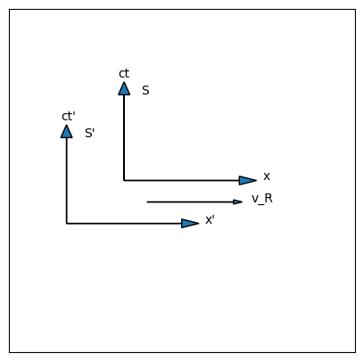
Fig. 3.2 Spacetime diagram of two reference frames in relative motion. The primed frame S’ (drawn to the left and down a little, although of course both reference frames are infinite in extent, and the origins may or may not coincide at a particular moment in time) is moving to the right at speed v_R, relative to the unprimed frame S, which is above and to the right. The x and x’ axes are defined to be parallel to the vector direction of v_R.

3.3. Examples of Displacement Four Vectors

The key to using this model of special relativity to describe physically real happenings is to be able to write down the displacement 4-vector for that happening. To do this, there must be two events occurring, events which both observers can detect. Then, each observer measures the physical displacements andthe time interval between the two events and converts them into the components of the displacement 4-vector as shown in Equation (3.1).

3.3.1. Muon Decay

For example, consider the following sequence of events: I am watching a pion travel along in a bubble chamber, leaving a track of bubbles. At some time and place, it decays into a muon. I know that something happens at that moment because the track of bubbles changes direction. The muon moves on for a while and then decays into an electron. Again, I know this happens because the bubble track changes direction. The two events are the change in direction of the tracks as shown in Fig. 3.3. Note that the figure on the left is a diagram of what happens in space, while the figure on the right is a spacetime diagram!

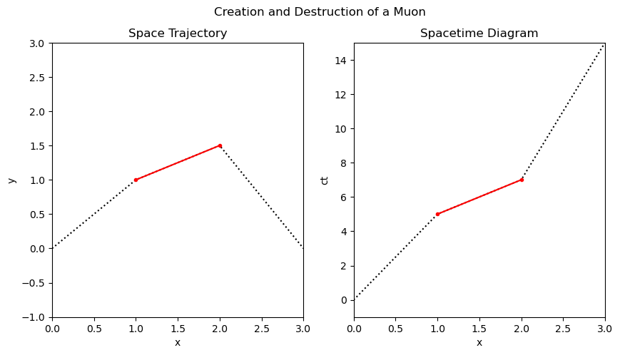
Fig. 3.3 Two diagrams to display the motion of particles. On the left, we have a plot of \(y\) vs. \(x\), which shows the trajectories of the particles. A pion enters from the lower left going up and to the right, turns into a muon and goes (mostly) straight to the right, and then turns into an electron that goes down and to the right. This diagram tells you nothing about how fast the particles are going, or how much time passes between the events. On the right, we have a spacetime diagram, which tells us nothing about the motion in the \(y\) direction on the left plot (the tracks on this diagram do not turn around), but does convey the velocity in the \(x\) direction (not the \(y\) or \(z\)!). Can you describe how this velocity component changes throughout this sequence of events? (Note: this is not realistic.)

If we consider the two events of the creation and disappearence of the muon, observers in the reference frame shown in Fig. 3.3 could measure the displacement and time duration between these events (and we can read them off the graph, albiet with no units), and then put them into the four-vector format:

(3.10)\[\begin{split}[dx_4] = \begin{bmatrix} icdt\\ dx\\ dy\\ dz \end{bmatrix} = \begin{bmatrix} i2\\ 1\\ 0.5\\ 0 \end{bmatrix}\end{split}\]

I put zero as the \(z\) displacement although technically we simply have no information about whether there was any displacement in the \(z\) direction.

3.3.2. Space ship

Often in SR problems, it is important to make a graph showing the events under consideration, and to indicate the relative motion of the reference frames, as in Fig. 3.2. This will help you visualize what’s happening and ensure that you set up your equations properly.

Consider a space ship that leaves the Earth and travels 4.2 LY to the star Alpha Centauri at a constant speed of \(\beta=0.75\). For this scenario, there are two reference frames that are of interest: the one that is at rest with respect to the space ship and another that is at rest with respect to the earth. The two events will be the departure from earth and the arrival at alpha centauri. The relative speed between these two observers is just the speed of the space ship in the direction of Alpha Centauri. The events can be diagrammed as shown in Fig. 3.4.

An observer that is at rest with respect to the Earth will measure (evenually – once all the rulers and clocks are returned and collated) a physical displacement in the \(x\)-direction of the distance between the Earth and Alpha Centauri: 4.2 light years. There will be no physical displacement in the \(y\) or \(z\) directions. There will be some time interval \(dt_\oplus\) that the Earth-based observer will measure for the trip. Since we know the velocity that the space is traveling with respect to the Earth, the time it takes to get to the star in the Earth’s reference frame is

\[dt_\oplus = \frac{dx_\oplus}{v_{\rm rocket}} = \frac{4.2~{\rm LY}}{0.75c} \rightarrow cdt_\oplus = 5.6~{\rm LY}\]

Note that \(cdt_\oplus\) has units of length.

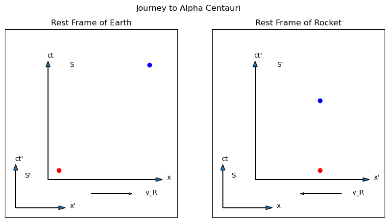
Fig. 3.4 Spacetime diagrams of two events in two different reference frames in relative motion. The left diagram represents the reference frame at rest with respect to the Earth. In this reference frame, the rocket leaves at the red dot on the lower left, travels 4.3 LY and arrives at the blue dot 5.6 years later. The primed frame in this case is the rest frame of the rocket. The right diagram shows the same two events from the primed frame: the Earth falls away behind the rocket while Alpha Centauri comes to meet it, while the rocket remains in the same place.

We can therefore write a displacement four vector in the reference frame at rest with respect to the Earth:

(3.11)\[\begin{equation} [dx_4]_\oplus = \begin{bmatrix} icdt_\oplus\\ dx\\ 0\\ 0 \end{bmatrix} = \begin{bmatrix} i5.6~{\rm LY}\\ 4.2~{\rm LY}\\ 0\\ 0 \end{bmatrix} \end{equation}\]

The observer aboard the space craft experiences these same two events: leaving the earth and arriving at Alpha Centauri. They both seem to occur just outside of the window of the space craft. There is no displacement between these two events! \(dx_{\rm rocket} = 0\). The observer aboard the space craft will measure some time interval, \(dt_{\rm rocket}\) between the time he sees the earth outside of his window and sees alpha centauri outside the window. The observer aboard the space craft measures a displacement 4-vector:

(3.12)\[\begin{equation} [dx_4]_{\rm rocket} = \begin{bmatrix} icdt_{\rm rocket}\\ 0\\ 0\\ 0 \end{bmatrix} \end{equation}\]

The Michelson-Morely experiment demands that the size of these two four-vectors be the same. Clearly, the observer on the spacecraft will measure a different duration for the trip than the clocks in the reference frame at rest with respect to the Earth will! Note this has nothing to do with the first observer being physically on the Earth – the \(dt_\oplus\) is measured by the infinite lattice of clocks at rest with respect to the Earth.

The sizes of the two four vectors are:

(3.13)\[\begin{equation} dx_\oplus^2 - (cdt_\oplus)^2 = -(cdt_{\rm rocket})^2 \end{equation}\]

Solve for \(dt_{\rm rocket}\):

(3.14)\[\begin{equation} dt_{\rm rocket} = dt_\oplus\sqrt{1-\left(\frac{dx_\oplus}{cdt_\oplus}\right)^2} = dt_\oplus \sqrt{1-\beta^2} \end{equation}\]

Note that the quantity under the square root will always be less than one, so the time interval on the rocket will always be less than the time interval in the Earth’s reference frame!

This is the famous Time Dilation, which will be explored in much more detail in Section 3.4. For now, it is sufficient to point out that the constant speed of light demands that the clocks attached to the lattice moving with the rocket measure a smaller time interval between these events than the clocks attached to the lattice that is at rest with respect to the Earth.

The Lorentz Factor: \(\gamma = \frac{1}{\sqrt{1-\beta^2}}\)

The quantity \(\sqrt{1-\beta^2}\) comes up so often it has a name: the Lorentz Factor, although it is usually more covenient to move it to the other side of the equation, since the clock on the rocket is the one at rest and therefore \(dt_{\rm rocket}\) is the smaller time interval. In this case,

(3.15)\[dt_\oplus = \frac{dt_{\rm rocket}}{\sqrt{1-\beta^2}} = dt_{\rm rocket}\gamma,\]

where \(\gamma \equiv 1/\sqrt{1-\beta^2}\) is the Lorentz Factor. The Lorentz Factor is always greater than or equal to one (equality in the case of \(\beta=0\) – no relative motion means the clocks will agree), so the clocks in the Earth’s frame will always measure a longer time interval, no matter the speed of the rocket.

Note

The relationships \(\gamma = 1/\sqrt{1-\beta^2}\) and \(\beta = \sqrt{1-1/\gamma^2}\) are very useful to know. When speeds start to get close to the speed of light, we often just write the speed as the Lorentz Factor, rather than converting it back to \(\beta\), or even \(v\). So it would be perfectly acceptable to just say something like “travelling with a speed of \(\gamma = 115\)”, even though technically \(\gamma\) is not a speed.

In the case presented here, \(\beta = 0.75\), so \(\gamma = 1.512\), and therefore the clocks on the rocket will measure a time interval of 3.7 years. This is a simplified version of the famous Twin Paradox, which adds the extra step of bringing the rocket back to Earth at the same speed, whereupon comparing the clocks shows that 7.4 years have passed on the rocket while 11.2 years have passed on the Earth. This may seem science fictional, but an experiment much like it has been carried out with jet planes going around the Earth in opposite directions, carrying extremely precise atomic clocks. The predicted rates of time dilation had to be modified to account for the fact that the planes were not inertial reference frames, but when correctly calculated, the predicted differences in the clocks were not different from the measured elapsed times, on the orders of a hundred nanoseconds! Look up descriptions of the Hafele-Keating Experiment for more details.

3.3.3. Clock on a Train

One more example of how you can use four-vectors to predict time dilation. Consider a clock, sitting on the floor of a train. It is linked to a laser, such that at a particular moment, it will cause the laser to flash. The laser is pointed at the ceiling of the train car, where a mirror reflects the laser beam right back down to the floor, where a detector stops the clock and therefore measures a time interval.

Example 3.2

The half-life for a muon is \(2.20 \times 10^{-6}\) seconds as ineasured in the rest frame of the muon. A particle accelerator, in the laboratory reference frame, produces a beam of a large number of muons, traveling at a speed \(v = 2.900 \times 10^8\) m/s as observed in the laboratory. Find the half-life of the muons as measured by the observer in the laboratory frame of reference.

The value of \(dt_0 = 2.20\times 10^{-6}\) s. What I am looking for is \(dt\). Equation (3.15) relates the two. What I need is to figure out a value for \(\beta\). Since \(\beta = v/c,\) it must be \(2.900\times 10^8\) m/s/(\(3.000\times 10^8\) m/s)=.9666. The Lorentz Factor is therefore \(\gamma = 3.906\), so \(dt = \gamma dt_0 = 8.59\times 10^{-6}\) s

To put this narrative into mathematical format, we define two events: the emission of the laser flash and the detection of the returning light. The emission and detection of the light happen at the same position in space, so the clock is at rest with respect to the events. Let us designate the time interval it measures as \(dt_0\). If the height of the train car is designated \(h\), then \(dt_0 = 2h/c\), since the laser beam moves at the speed of light.

Now consider that the train is moving along horizontal tracks at a speed \(v\), relative to the ground. Standing on the ground is another observer with a clock, and this observer starts and stops their clock at the same events (note that we are not worrying about the time it takes light to travel from the train to the person on the ground – we are using these two clocks to stand in for the imaginary infinite lattice of rulers and clock that make up our conceptual reference frames). We say this person measures a time interval \(dt\) between the emission and detection of the light. How does \(dt\) compare with \(dt_0\)?

First, there are three relevant events: the light beam is emitted upward, it reflects off a mirror on the ceiling, and it returns to the detector next to the clock. These three events happen, so they must happen in all reference frames. Since according to the person on the ground, the train is moving, the mirror will be a distance \(vdt/2\) along the track when the light hits it, and \(vdt\) further along when the light returns. In the ground’s reference frame, the light must therefore follow a triangular path, if it is to bounce off the mirror and return to the detector. An interactive animation of this situation is shown in Fig. 3.5. Run the simulation a few times for different train speeds before continuing, to make sure you are correctly visualizing the situation.

Fig. 3.5 Animation of a laser clock on a train. Use the slider to set the speed of the train and then click the button to run the animation. The white ball represents the pulse of light from the laser. It will travel from the floor of the train, reflect off the ceiling, and return to the floor. The readout to the lower left shows the time elapsed while the laser is moving. The calculations use \(c=1\), so this is also the distance the laser beam travels. Try it first with \(\beta=0\) and see the ball go straight up and down. The height of the train is 6, in these units, so you should see the time of flight as 12. Try increasing \(\beta\) and run it again, to see how the time and distance increase. An observer on the train would only ever measure the \(\beta=0\) case.

This is the essence of time dilation: if the light is to travel a longer path (the hypoteneuse of a triangle will be longer than the vertical side) at the same speed, it must take more time to do so. The length of the horizontal side of the triangle is the distance the train moves, \(vdt/2\) for each of the away and back segments. The diagonal path is therefore of length \(2\sqrt{h^2+(vdt/2)^2}\). The time interval the person on the ground will measure is thus:

\[dt = \frac{D}{c} = \frac{2\sqrt{h^2+(vdt/2)^2}}{c}\]

Substitute in \(h=cdt_0/2\) and square both sides to get

\[dt^2 = \frac{4(cdt_0/2)^2+(vdt/2)^2}{c^2}\]

The four cancels, and if we multiply both sides by \(c^2\),

(3.16)\[c^2dt^2 = (cdt_0)^2+(vdt)^2 \rightarrow dt^2(c^2-v^2) = c^2dt_0^2\]

which means

(3.17)\[dt = dt_0\frac{1}{\sqrt{1-(v/c)^2}} = \gamma dt_0,\]

which is the same as Equation (3.15)! Just as with the rocket, the clocks that are associated with the reference frame at rest with respect to the two events (the clocks on the train) measure a shorter time interval than the clocks in the reference frame where these two events are not in the same place. The clock on the ground will measure a longer time interval than the clock on the train by a factor of \(\gamma\). From the point of view of the person on the ground, the clock on the train is therefore running slow, so often time dilation is summarized as “moving clocks run slow.” However, see Section 3.4 for an exploration of important ways in which this statement is misleading and easily misunderstood.

You can also express this example through the formalism of the displacement four vectors, and in fact, Fig. 3.4 will serve just as well to represent this situation. In the reference frame of the train, the events of the light being emitted and then being detected are in the same place, so in the context of Fig. 3.4, the train frame is the primed frame on the right. The reference frame at rest with respect to the ground is the unprimed frame on the left. The red dot is the emission of the light and the blue dot is the detection of the light. The displacement four vector in the train frame would be:

(3.18)\[\begin{equation} [dx_4]_{\rm train} = \begin{bmatrix} icdt_0\\ 0\\ 0\\ 0 \end{bmatrix} \end{equation}\]

while the displacement four vector from the ground’s reference frame is

(3.19)\[\begin{equation} [dx_4]_{\rm ground} = \begin{bmatrix} icdt\\ vdt\\ 0\\ 0 \end{bmatrix} \end{equation}\]

Since the size of these four-vectors must be the same, that means

\[-c^2dt_0^2 = -c^2dt^2+v^2dt^2,\]

which is exactly the same as Equation (3.16), which means that, again, \(\boxed{dt = \gamma dt_0}\).

Despite what seem to be completely different contexts, the underlying physics of the rocket and the train are exactly the same, because the rules of time are the same.

3.4. Time Dilation

Time Dilation is one of the most important, and most confusing, demands of the theory of Special Relativity. The principle is often characterized by the phrase “moving clocks run slow”, but I find this phrase confusing, as all clocks could be in motion, relative to something else. In the examples above, the Earth is moving in the rocket’s frame of reference, and the ground is moving in the train’s frame of reference, so which clock is moving? If “moving clocks run slow”, could we determine which clock is running slow, and then that would tell us which clock is really moving?

Time Dilation: a set of clocks in a reference frame at rest with respect to two events will measure the shortest possible time interval between those two events.

A more precise formulation of the principle is “a set of clocks in a reference frame at rest with respect to two events will measure the shortest possible time interval between those two events.” Specifying which frame of reference has the two events at rest (at the same location in space) breaks the symmetry and avoids the confusion as to which clock is moving. There is only one relative reference frame where the two events are at rest. In this reference frame, the time interval is a minimum. Switching into any other reference frame will result in clock measurements that yield a longer time interval. In the rocket example, the events of leaving Earth and arriving at the distant star are in the same location from the rocket’s point of view, not the Earth’s. The light returning to the floor of the train is at the same location on the train, not from the reference frame of the ground. The rocket and the train will therefore measure the shortest time interval.

This shortest time interval, being unique, also gets a name, and is called the proper time interval, and is often designated \(dt_0\). If you are not clear on which clock is moving, draw a spacetime diagram and see whether the two events you are considering are in the same place. Often, the confusion arises because someone is not carefully considering what the two events in question actually are, and they mistakenly compare two different time intervals, rather than the same interval in different reference frames.

Note

Make sure you understand that nothing in SR makes any demands on what kind of clock is being used to make the measurements. Time dilation is not a mechanical effect of the particular clock making the measurements. Any spatially repeating system (rotation, vibration, oscillation) can act as a clock, and all of them will measure time dilation. It’s a necessary implication of the two postulates of Relativity, a property of time itself, not a description of gears winding down or some other feature of a particular kind of clock.

It is worth reminding one’s self at this point that we are not demanding that time have some kind of universal flow that somehow changes when you change the speed of your reference frame. Relativity demands you let go of the Newtonian idea of a universal grid of space and time that underlies our lattice of rulers and clocks and is there whether we have a lattice or not. In SR, the measurements of the clocks is time. If you still think of some kind of universal time flow that changes its rate in different frames, you are still hanging on to aspects of the classical way of thinking that you need to release.

The local nature of the effect of time dilation on time intervals is shown in Fig. 3.6, which is an animated adaptation of a graph in the delighful [Takeuchi, 2010]. The figure shows a spacetime diagram with four particular events marked as colored dots. In the initial reference frame, these four events are at two different locations: the first and last are to the right of the second and third. The events are spaced evenly in time, with \(c\Delta t\) being 0.2 units between each successive pair of events. Horizontal colored lines show where the clock readings would be read off the time axis, and the clock reading numbers themselves are indicated in white boxes to the left of the axis.

By moving the slider to the right or left, you can have the yellow arrows shift to indicate the set of events that would lie on the axes in reference frames in relative motion. The colored lines will shift to indicate where the clock readings for the new axes would be, and the clock readings themselves will change to indicate which events on the new time axis are simultaneous with the four events.

If the flow of time were some universal thing; something that changed according to your frame of reference but still existed everywhere, the numbers in the boxes would maintain the same differences. However, if you shift all the way to the left, you can see that the second event happens more quickly after the first than the fourth does after the third. If you shift the slider all the way to the right, it’s the last two events that happen in quicker succession than the first two events.

The conclusion is inescapable: the time interval between two events depends on where and when the pairs of events are, and not some kind of universal rate of the flow of time. In the next few chapters, we will explore more productive ways to think about the relationships between space, time, and motion, but the most important step to make now is to let go of the idea of a single, universal, underlying space that exists independent of our measurements of it, and a flow of time that functions independent of space and our motion through it.

Fig. 3.6 Interactive animation of time intervals. Four events are indicated in different colors. A slider changes the relative velocity to another reference frame. The four numbers in the white boxes indicate the clock readings along the time axis at the events that are simultaneous with the four colored events in the relatively moving reference frame. The key takeaway is that while the four events are evenly spaced in time in the original frame (\(\beta_R=0\)), the time intervals between events do not stretch identically in every other frame. Time dilation is not a universal, uniform, change in the “flow of time”.

3.5. Problems

1. An experimenter measures the following physical changes between two events \(dx = 1.00\) m, \(dy = 0.300\) m, \(dz = -0.100\) m, and \(dt = 6.00\) ns. Write down the displacement 4-vector for these events. Find the size of this displacement 4-vector.

2. A beain of a certain type of elementary particle travels at a speed of \(2.85\times 10^8\) m/s with respect to the lab reference frame. The average life time of the particle is measured to be \(2.50 \times 10^{-6}\) s in the lab. Draw the space-time diagram of the two events (creation and decay of the particle) as seen by an observer at rest with respect to the lab. Draw the space-time diagram of the two events as seen by an observer that is at rest with respect to the elementary particle. What is the particle’s average life time in the rest frame of the particle?

3. An observer measures the displacement 4-vector between two events to be:

\[\begin{split}[dR_4] = \begin{bmatrix} i 3.00~{\rm cm}\\ 0.0~{\rm cm}\\ 2.0~{\rm cm}\\ 0.0~{\rm cm} \end{bmatrix}\end{split}\]

Is this observer in the rest frame of the events? Why? Find the time interval measured by this observer. How fast is the object, described by this displacement 4-vector, traveling? In what direction is it traveling?

4. When working with equations of relativity theory, physicists routinely set the speedof light \(c = 1\) (with no units!) as a matter of convenience. Find the value and units of a time interval of \(1.00\) seconds in this system of units. In this set of units, what is the speed of sound in air, the speed of the earth in its orbit about the sun and the speed of a neutrino?